Abstract
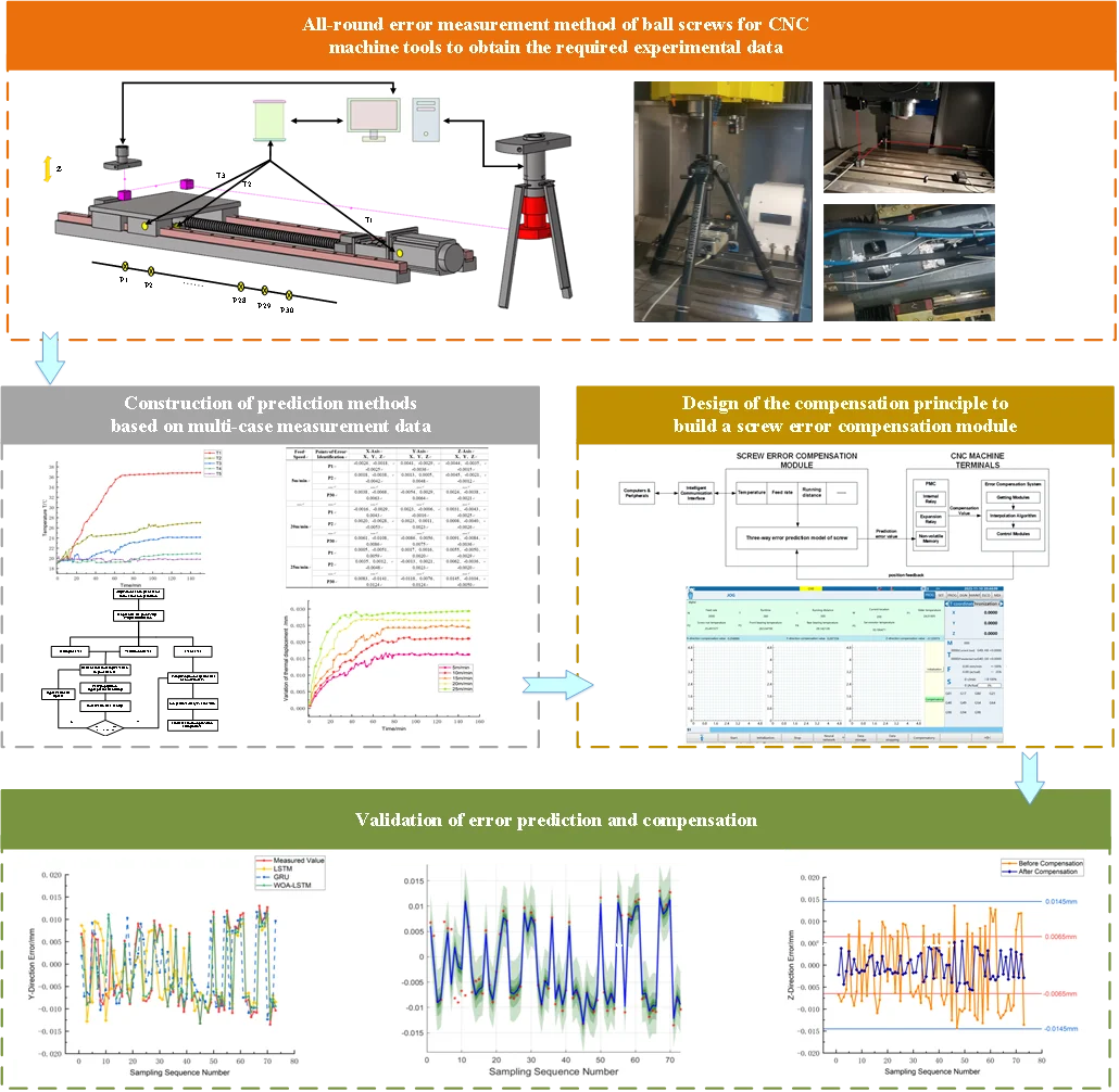
Considering the detrimental impact of thermal phenomena on the geometric precision of machine tools, a machine tool ball screw’s omni-directional error model is created using the LSTM neural network algorithm. Subsequently, the machine tool ball screw's omni-directional error compensation module is devised by combining the core functions of the Huazhong numerical control system with the visual programming environment of QT and the numerical computation capability of Matlab. To enhance the practicality and accuracy of the compensation model, this study has employed the Whale Optimization Algorithm (WOA) to optimize the parameters of the LSTM model. This has resulted in an improvement in the model's generalization ability and prediction performance, making it more effective. During the experimental validation phase, the -axis error of the machine tool was practically operated and analyzed using the compensation method. Results manifestly show that, after employing the compensation method, the peak amplitude of the -axis error fluctuations have been notably curtailed to ±0.006 mm – a considerable reduction compared to the initial error bandwidth of ±0.0145 mm. These empirical findings substantiate the efficacy of the proposed compensation strategy in substantially boosting the machining precision of products, thus furnishing a substantial and instructive benchmark for future inquiries into CNC machine tool error compensation technologies.
1. Introduction
Ball screws play a critical role in the manufacturing industry, but their reciprocating motion in CNC machine tools generates frictional heat, leading to thermal expansion [1]. This expansion phenomenon subsequently induces shifts in the relative positioning of the cutting point, ultimately impacting the precision of workpiece machining processes [2]. While conventional screw error compensation technology in the axial direction is effective, radial compensation still needs improvement, especially for the two ends of the fixed screw structure [3]. Against this backdrop, the present study focuses its investigative efforts on the development and resolution of the multifaceted challenge posed by omni-directional error compensation necessitated by thermal effects in dynamically functioning screws.
In recent times, research on thermal error modeling methods based on the principle model (PBM) and empirical model (EBM) [4] has been limited due to their low prediction accuracy. Consequently, a range of thermal error modeling techniques have been proposed by scholars both domestically and internationally; among these, the application of deep learning to error compensation has progressively grown to become a research hotspot in the field. For instance, Li Bin et al. [5] harnessed a wavelet neural network optimized via genetic algorithm to build a thermal error model for CNC machine tools, which they experimentally validated for its superior attributes, including accuracy, resistance to interference, and robustness. Similarly, the four-layer neural network architecture proposed by Pu-Ling Liu et al. [6] showcased commendable precision and resilience in predicting thermal errors during machining operations. Moreover, various scholars – such as Hu Shi et al. [7], Guo Qianjian et al. [8], Li Guangbao et al. [9], and Li et al. [10] – have independently enhanced the predictive and compensatory capabilities of error models by implementing different optimization algorithms and neural network architectures.
Amidst the ongoing evolution of error prediction technologies, a deeper understanding of thermal error characteristics becomes increasingly crucial. Li S. S. et al. [11] employed the finite element method to scrutinize the thermal attributes, vibrational modes, and natural frequencies of a motor spindle in both steady-state and static conditions. Li Yi et al. [12] conceptualized and experimentally substantiated an efficient water-cooling system tailored for motor spindles. H. Qu et al. [13] systematically reviewed the principal sources of thermal errors and prevailing control strategies while envisioning prospective research directions. Parallel to this, advancements in error compensation technology significantly contribute to enhancing machining precision. Lu Chengwei et al. [14] presented a feature decomposition-based key geometric error analysis and compensation strategy applicable to five-axis CNC machine tools, offering detailed analyses and efficacious remedies for critical geometric errors. Li et al. [15] developed a thermal error modeling and compensation technique for heavy gantry machine tools, demonstrating marked effectiveness, with the mean error diminishing from 101 microns to 13.5 microns. Chen Guo-Hua et al. [16] constructed a volumetric error model for machine tools grounded in Abbe error theory, incorporating it into the system to realize error compensation, which they confirmed by contrasting tool accuracy pre- and post-compensation.
Synthesizing these studies, preventative and compensatory measures constitute the dual mainstream strategies for coping with thermal error problems [17]. Nevertheless, preventive measures are often costly and are limited by technological constraints. Coupled with the less-explored issue of errors emanating from the fixed state of CNC machine tool screws’ ends, this study innovatively introduces an omni-directional error compensation method targeting the screw structure's interaction with heat sources. This novel approach addresses a gap in the literature and promises significant improvements in coping with thermal error challenges.
2. Principle and methods
2.1. Principle analysis of LSTM
Deep learning is a widely used machine learning technique that combines underlying features to reveal complex patterns [18]. Harnessing high-capacity training algorithms on extensive datasets, this technique excels at discerning sophisticated relationships.
Among its variants, Long Short-Term Memory (LSTM) [19] represents a refined rendition of recurrent neural networks, explicitly designed to mitigate the notorious challenges of gradient disappearance and explosion inherent in conventional recurrent architectures. The LSTM network state is regarded as a dynamic system, where a memory cell and three gate structures (input gate, output gate, and forget gate) constitute a long and short-term memory unit. A graphical depiction of these gates is provided in Fig. 1, elucidating their operational dynamics within the LSTM structure.
In LSTM, the update of each state variable follows the following formula:
The oblivion gate determines the degree of oblivion of the hidden cell state at the previous moment by using Eq. (1), where denotes the output of a sigmoid function that proportionally “obliviates” the previous hidden state based on the current input :
The filtering of valid information is indicated by the in Eq. (2), and each component is given a weight ranging from 0 to 1. The likelihood that a component will be chosen and added to the unit state increases with weight:
Eq. (3) delineates the formulation of a candidate state vector , wherein the utilization of a hyperbolic tangent activation function () plays a pivotal role. This function restricts the output spectrum to the interval [–1, 1], a characteristic that fortifies the LSTM's resilience against the common issues of vanishing and exploding gradients, thereby preserving the inherent expressiveness of the encoded information.
Fig. 1Schematic diagram of LSTM unit structure
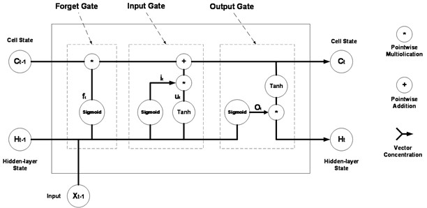
The activation function () behaves as:
In addition, Eqs. (2) and (3) together form the mechanism for the operation of the input gate (memory gate), which determines whether the data at time step is integrated into the cell state.
At time step , the cell state undergoes an update governed by Eq. (5), where the retention or forgetting of past information is initially modulated by a sigmoid function, utilizing the output from the previous time step and the input at the current instant. A sigmoid value of 1 indicates a strong retention of the previous state , while a value of 0 indicates complete forgetfulness of the previous state:
Eqs. (6) and (7) expound upon the operative mechanism of the output gate. First, a sigmoid function is engaged to sieve out pertinent information from a composite vector , which consolidates the current input and the output from the immediately preceding time point. Subsequent to this, the current cell state is transformed onto the interval (–1, 1) through the application of a hyperbolic tangent function , thereby shaping the ultimate output value that encapsulates the processed temporal information.
In the above equation, at time , represents the input data, represents the state of the hidden layer, + represents the superposition operation, represents the matrix weight, represents the offset, represents the sigmoid function, and the symbol represents the vector outer product. The usual LSTM network structure is shown in Fig. 2.
Fig. 2Schematic diagram of long short-term memory network
2.2. WOA optimization algorithm
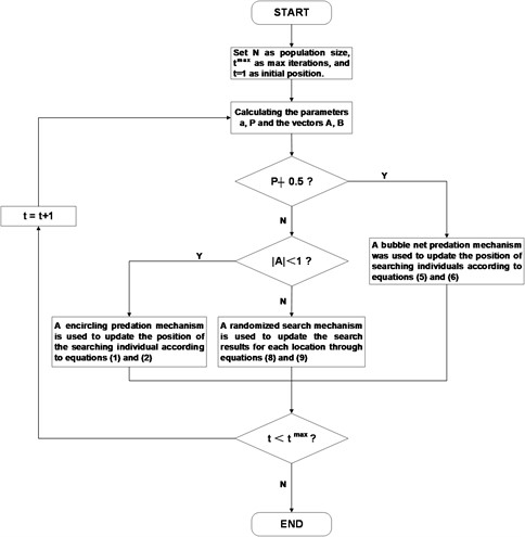
The WOA algorithm is designed to optimize a problem by imitating biological strategies used in the hunting behaviour of humpback whales, such as encircling predation and bubble net predation. Within this framework, each artificial humpback whale embodies a potential solution, and its position iteratively evolves to approach the global optimum:
The strategic essence of the encircling predation strategy is instantiated in Eq. (8) and (9), wherein, once a prevailing global optimum is identified, the remaining members of the population progressively converge towards it in accordance with predefined rules. Herein, and denote dynamically tuned coefficient vectors contingent upon the iteration count , while stands for the present initial position vector of an individual whale agent. The position adjustment process is judiciously guided by the utilization of the absolute value operator and the Hadamard product (element-wise multiplication) operator , ensuring a systematic movement toward the most promising areas of the search space:
Throughout the iteration process, the computation of vectors and follows Eqs. (10) and (11), where decreases linearly to zero with the number of iterations and and are random numbers in the interval [0, 1]:
Eqs. (12) and (13) describe the equation of a logarithmic spiral that is used to calculate the position update of whales and their prey during bubble net predation. In the equation, represents the distance between the current individual and the current optimal solution, is the spiral shape parameter, and is a random number uniformly distributed between [–1, 1]:
Eq. (14) shows the process of WOA selecting different predation strategies based on the probability P, which is a random probability in the range of [0, 1]:
In Eqs. (15) and (16), when 1, the exploratory agents not only gravitate towards the identified optimal solution but also recalibrate their positions in relation to the distances from randomly chosen peers, thereby instigating a broader scope of random search. Here, denotes the distance between the current individual and the random individual, and is the position of the random individual.
To conclude, the WOA algorithm ingeniously amalgamates a biomimetic heuristic with a pliable probabilistic decision-making process, which guides the searching individuals to effectively traverse the solution space in the iterative process to find the globally optimal solution. The comprehensive workflow of the WOA algorithm is visually depicted in Fig. 3, which lucidly illustrates the algorithm’s entire operational sequence.
Fig. 3Flowchart of WOA algorithm optimization
2.3. Model framework
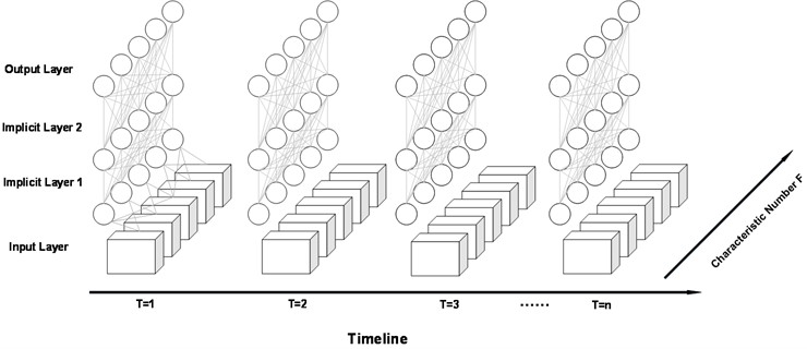
Since the ball screw error data manifest temporal correlations and continuity, and are notably influenced by the thermal dynamics of the machine tool, this study adopts an LSTM network to examine the data within a dynamic time series framework, aiming to capture their intricate spatiotemporal properties and deliver precise thermal error predictions [20].
The construction of the three-dimensional error prediction model for the ball screw encompasses several stages: data preprocessing, model architectural setup, hyperparameter tuning, and model testing and evaluation.
During the preprocessing phase, a variety of multivariate data are gathered and meticulously organized, concatenated, and normalized, encompassing the running distance, servomotor temperature, slider temperature, screw nut temperature, and the three-directional errors (, , ). Among them, the preset temperature data includes motor mount temperature, ball screw nut temperature, and guideway slider temperature, with weights of 70 %, 20 %, and 10 %, respectively. Meanwhile, the running distance, sampling position, and preset temperature data are taken as model input parameters, and the three-way error is taken as output parameters. The dataset is divided into 70 % as the training set, 10 % as the validation set, and 20 % as the test set.
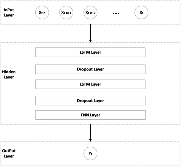
The model architecture is depicted in Fig. 4. Its input layer contains the input sequence at time t and its previous period, while the output layer represents the value of the three-way error of the ball screw predicted by the model at time . Multiple hidden layers are set up inside the model, including the FNN layer, LSTM layer, and dropout layer, with a serial connection of two LSTM layer-dropout layer pairs culminating in a fully connected FNN layer. Among them, the LSTM layer mainly undertakes the task of extracting key features from the input sequence and maintaining the internal state.
Fig. 4Framework diagram of predictive modeling
In order to obtain optimal performance from the LSTM model during training, it is necessary to adjust its configuration and parameter tuning. This involves finding the best combination of hyperparameters, such as the learning rate, number of hidden neurons in the LSTM layer, regularization coefficient, and number of training rounds, through several iterations. However, traditional optimization algorithms may be computationally expensive and inefficient, so this study uses the WOA algorithm. It is chosen for its fast convergence and excellent global optimal solution search capability. Moreover, to guarantee the gradient stability of the screw’s three-way error prediction model, the uniform initialization method [21] is employed to initialize model parameters. The LSTM model adopts the tanh and sigmoid functions as activation functions, complemented by the Adam optimization algorithm [22] for parameter adjustment, aimed at minimizing the loss function.
In the final stage of model assessment, this study primarily utilizes the root mean square error (RMSE) as the primary metric for gauging prediction accuracy, complemented by the mean absolute error (MAE) to quantify the magnitude of disparity between the predicted and actual values:
2.4. Training of algorithm
In this study, a ball screw three-way error prediction model is shown in Fig. 5. During the training process, the dataset is divided into small batches. In each batch, the model receives a set of input sequences and calculates the gradient of the loss function through a backpropagation algorithm. These gradients are then used to update the model parameters to minimize the loss function. On this basis, the optimizer exploits the computed gradients to refine the model parameters, and this iterative training process persists until a convergence criterion is met. Of particular note, the Dropout layer is used to prevent overfitting by implementing an early stopping strategy.
Fig. 5Flowchart of Three-way error prediction of ball screws
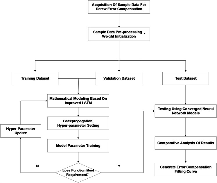
As per the previously discussed Section 2.3, the WOA algorithm is used to optimize the best hyper-parameter combination for the experiment. Since the training sets are different, the set hyperparameters are also different. Ultimately, following rigorous training and meticulous parameter optimization, the high-performing LSTM neural network model was successfully integrated into a custom-built screw error compensation module. This integration enables the accurate prediction and efficacious compensation of the ball screw's three-directional errors in practical application contexts.
2.5. Training of algorithm
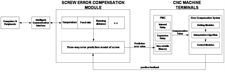
The error compensation function of the CNC machine tool is a result of integrating various technologies such as Fast Ethernet data interaction technology, sensor technology, real-time control system, and adaptive control technology. The principle of the error compensation system is illustrated in Fig. 6. The error prediction value, computed by the three-way error prediction model of the ball screw, is quickly stored in the non-volatile memory of the programmable machine controller (PMC) through data interaction. When the machine tool error compensation system interacts with the PMC, the data is transferred to the built-in interpolation system. The data is then adjusted by an internal interpolation algorithm that converts the compensation value into an interpolation step, which is transmitted to the interpolator to correct the interpolation vector.
Fig. 6Schematic diagram of ball screw error compensation
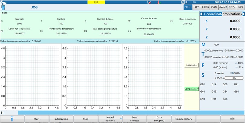
This study aims to address the issues of cumbersome testing and low efficiency of CNC systems by developing a ball screw error compensation module. The module is designed to be highly stable, personalized, and user-friendly, with a high degree of human-computer interaction. It is developed using the secondary development of QT software and is designed, developed and debugged in a Win environment, which includes: module function definition, interface design, operation logic processing, parameter configuration, motion control, etc. The module interface is shown in Fig. 7.
QT introduces the signal and slot mechanism to enhance the communication function between the system and interpolator, making the interaction between system components more convenient and flexible. The signal and slot mechanism allows communication and interaction between components through a reaction-slot (slot) approach, making it easy to communicate between different threads and achieve real-time data transfer and synchronization. This improves the response speed and efficiency of the system. In the secondary development of the ball screw error compensation module, the sensor data can be sent as a signal and then connected to the slot function of the interpolator to realize real-time data interaction and control.
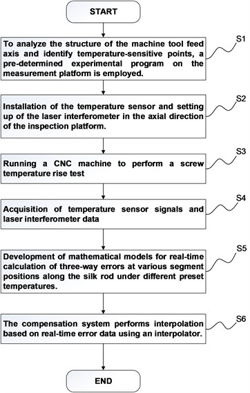
2.6. Construction of Omni-directional error compensation method
The omni-directional error compensation method is to address the issue of thermal error resulting from thermal deformation when the ball screw’s two ends are fixed. The detailed implementation process is illustrated in Fig. 8. To accomplish this, the method employs both QT and MATLAB software for secondary development of the CNC system, as well as to establish a three-way error prediction model for the ball screw.
Fig. 7Ball screws error compensation module interface
During this process, data about the ball screw's movement is collected, including its real-time position, feed speed, running time, running distance, and temperature at the sensitive point. These data are then fed into a WOA-LSTM prediction model, which has already been established. After performing mathematical calculations and fitting the model, the system obtains the three-way errors (, , ) at the real-time position of the machining platform. These errors are then sent to the interpolator, which uses the values to generate control signals and adjust the servo motors accordingly. The main goal of this method is to use feedback control to ensure that the tool or workpiece moves as close as possible to the desired trajectory, thereby improving machining quality and accuracy. By using real-time error data, interpolation is achieved through the interpolators in the compensation system. This system ensures that the machine is stable when handling complex workpieces.
For data acquisition, it is necessary to preset an experimental program for the acquisition process and use the control variable method. The experimental program must include adjustments to motor speed and machining platform feed speed, presetting segmented measurement points, and developing a temperature rise test program. The segmented measurement points are preset by dividing the feed ball screw of the CNC machine tool into multiple parts according to the same spacing (), and dividing them into different three-way error measurement areas. In each region, the point at /2 is set as the measurement point. The temperature rise test program involves writing G-code to control the reciprocating motion of the measuring platform feed system within a given distance (S) to mimic the actual machining state of the CNC machine tool and generate localized high temperatures. During this process, the feed axis ball screw of the CNC machine tool deforms due to thermal expansion.
During data acquisition, the CNC machine's three axes were run without any load and stopped for 3 seconds at 1/2 of each pitch, /2, in accordance with the ISO international standard [23]. During the halt period, a laser interferometer was used to measure the three-way error data of the current segmented position of the ball screw, while a temperature sensor collected data on the ball screw's temperature during operation, including the temperature of the servo motor, slide, and ball screw nut. After collecting the data, they were preprocessed and integrated into the dataset required for the model.
Fig. 8Flowchart of Omni-directional error compensation method
3. Thermal error measurement experiment
3.1. Construction of experimental environment
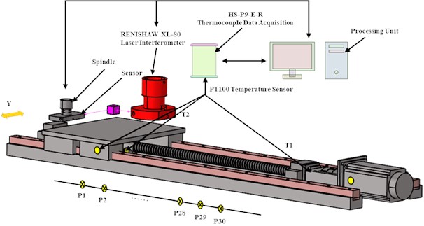
This study zeroes in on the thermal error issue pertaining to the feed screw within the S7H composite machining center, employing high-precision instruments such as PT100 temperature sensors, an HS-P9-E-R temperature acquisition device, and a Renishaw XL-80 laser interferometer for experimental execution. Notably, the detailed layout arrangement of the -axis is graphically depicted in Fig. 9, whereas the positioning of the laser interferometer for the - and -axis screws is tailored according to the experimental requisites.
Concurrently, in pursuit of obtaining a representative ambient temperature, two additional temperature measurement points, T4 and T5, are symmetrically installed on both the inner and outer surfaces of the machine, with their mean value serving as the ambient temperature reference. The initial positioning error of the machine is accurately measured by a laser interferometer [24]. Given that the total length of the screw measures 600 mm, it is uniformly divided into thirty sections, each segment of length 20 mm, with an error detection point established at the midpoint of every segment for meticulous error analysis.
In light of the heat dissipation patterns intrinsic to the ball screw, temperature sensors are strategically positioned in thermally sensitive regions such as the screw nut, guideway slide, and servo motor, designated as monitoring points T1, T2, and T3, respectively. These PT100 resistance temperature sensors [25] boast a ±0.3 °C high-precision measurement capability and operate across a wide temperature range from –200 °C to 300 °C.
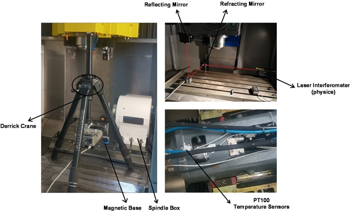
The configuration of the laser interferometer system at the ball screw is elucidated in Fig. 10, comprising elements such as the interference head, refractor, reflector, stable tripod, and other components. Initially, the robust tripod is stationed atop a dedicated support pedestal, facilitating the mounting of the laser interferometer's main apparatus to ensure that the interference head is aligned in the zero-coordinate horizontal plane of the machine tool's working platform, thus guaranteeing the precision of the measurement reference point. Subsequently, an adjustable support rod is affixed to the -axis column using a magnetic base, allowing it to ascend and descend in unison with the -axis motion. Upon this rod, a reflector is securely attached, which tracks the vertical displacement of the -axis and fundamentally serves to receive and redirect the laser beam horizontally from the laser interferometer.
Fig. 9Schematic diagram of thermal error measurement setup
Simultaneously, a refractor mirror is prescriptively positioned on a support bar, its exact placement lying at the geometric intersection of the laser interferometer’s -axis extension line and the principal axis of the machine tool – this position remains invariant with the worktable’s movements. The refractor's function is to collect the horizontally emitted laser beam from the interferometer, refract it towards the reflector, and thereafter intercept the laser beam returning from the reflector, thereby ensuring it is vertically impinged upon the receiver aperture for meticulous optical analysis and measurement.
Fig. 10Arrangement of laser interferometer
3.2. Protocol for measurement experiment
The experimental protocol unfolds in the following sequential phases:
1) Precise temperature sensors are strategically placed in zones of the machine tool apparatus that are susceptible to significant temperature fluctuations. At the same time, key error detection points are marked, and the distribution of positioning errors at each point is accurately quantified using a laser interferometer.
2) Proceeding to the temperature rise experiment, the feed system of the machining center was operated with its cooling mechanism deactivated, while the worktable executes reciprocating motions along the feed axes at a steady speed of 10 meters per minute. The temperature data from the sensors are recorded in real-time. When the temperature approaches a predetermined threshold, the feed rate is reduced, and there is a mandatory pause of 5 seconds at each error detection point to collect relevant data.
3) Throughout each pause interval, the three-dimensional error data were meticulously captured at each segment along the ball screw's length using a laser interferometer. Simultaneously, a continuous surveillance and logging of the comprehensive temperature data took place, encompassing the servo motor, slider, and screw nut temperatures.
4) To examine the impact of varying feed speeds on error magnitudes and temperature changes, the experiment includes a stepped increase in feed rates, starting from 5 meters per minute up to 25 meters per minute. The previous experimental procedures are repeated rigorously at each feed speed to ensure comprehensive data collection and credibility.
3.3. Data analysis
Under ambient room temperature conditions, the ball screw is driven to reach thermal equilibrium status at a feeding velocity of 10 m/min, which is considered achieved when the temperature increase approximates around 95 %. The perusal of experimental data reveals that the internal and external ambient temperatures of the machine tool stabilize at approximately 20 °C. The -axis feeding system exhibits a characteristic pattern of rapid initial temperature escalation followed by a gradual slowdown and eventual stabilization. Specifically, the temperature escalates swiftly during the initial 70 minutes before plateauing around 110 minutes later. The temperature variation curves for the three temperature-sensitive points and the measuring points on the inner and outer surfaces of the machine tool are presented in Fig. 11. Owing to the semi-enclosed nature of the motor end, which leads to relatively inferior heat dissipation conditions, the temperature at measurement point T1 (the motor) peaks and stabilizes at around 36 °C. Following this, the screw nut at measurement point T2 attains a steady-state temperature of about 27 °C, and the slider at measurement point T3 records the lowest temperature, stabilizing at approximately 24 °C. This disparity is attributed to the slider's mobility with the feeding system and larger air contact surface area, resulting in more efficient heat dissipation. The elevated temperature of the screw nut compared to the slider is mainly due to the heat generation from the nut-pair interaction. Ultimately, all temperature data were collated, and the temperatures at T1, T2, and T3 are preset to the temperature record value according to the weights of 70 %, 20 %, and 10 %, respectively.
Once the temperature within the monitoring system reaches the pre-established threshold, a laser interferometer is utilized to quantify the thermal error, which is calculated as the difference between the measured values at each time interval and the initial positioning error.
The radial offsets and expansion deformations caused by mechanical forces and thermal influences manifest positively along the positive direction of the system coordinates. Fig. 12 illustrates the variations in thermal error at a representative error detection point under different feed speeds, effectively demonstrating the substantial correlation between feed speed and the thermal error of the ball screw – specifically, an increase in feed speed results in a commensurate rise in thermal error. Hence, a judicious decrease in feed speed can be instrumental in mitigating thermal error.
Table 1 encapsulates select experimental error data, indicating that the three-way error at the ball screw measurement points closer to the motor end is substantial, particularly beyond point P26, where the maximum error can reach up to ±14.59 μm. It is noteworthy that the initial positioning error registers negatively and veers in both positive and negative directions, which can be attributed to the fixed mounting of the screw’s two ends.
Fig. 11Temperature variation curves at various positions under a feed rate of 10 m/min
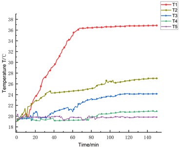
Fig. 12Thermal error variation curve under different feed speeds at the same position
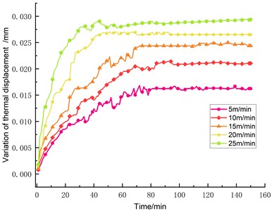
Table 1Three-axis errors at varying inspection points (mm)
Feed speed | Points of error identification | -Axis | -Axis | -Axis |
, , | , , | , , | ||
5 m/min | P1 | –0.0026, –0.0018, –0.0025 | 0.0041, –0.0029, –0.0036 | –0.0044, –0.0035, –0.0015 |
P2 | 0.0018, –0.0038, –0.0042 | 0.0013, 0.0005, 0.0048 | –0.0045, –0.0021, –0.0012 | |
… | … | … | … | |
P30 | 0.0038, –0.0068, 0.0063 | –0.0054, 0.0029, 0.0064 | 0.0024, -0.0038, –0.0021 | |
… | … | … | … | … |
20 m/min | P1 | –0.0016, –0.0029, 0.0043 | 0.0023, –0.0006, –0.0016 | 0.0031, –0.0043, –0.0025 |
P2 | 0.0020, –0.0028, –0.0053 | 0.0023, 0.0011, 0.0023 | 0.0008, –0.0040, –0.0026 | |
… | … | … | … | |
P30 | 0.0061, –0.0108, 0.0086 | –0.0086, 0.0056, 0.0075 | 0.0091, –0.0084, –0.0036 | |
25 m/min | P1 | 0.0005, –0.0051, 0.0059 | 0.0017, 0.0016, 0.0020 | 0.0055, –0.0050, –0.0029 |
P2 | 0.0035, 0.0012, –0.0048 | –0.0013, 0.0021, 0.0023 | 0.0062, –0.0036, –0.0020 | |
… | … | … | … | |
P30 | 0.0083, –0.0141, 0.0124 | –0.0118, 0.0076, 0.0124 | 0.0145, –0.0104, –0.0050 |
4. Experimental results analysis and model validation
4.1. Experimental analysis of predictive modeling
In the present study, a series of error measurement experiments were systematically conducted on an S7H composite machining center under diverse preestablished temperature and feed rate scenarios, thereby generating datasets essential for model training and validation purposes.
Subsequent to this, the determination of model parameters was executed by identifying the most optimal loss function on the validation dataset. The efficacy of the model was further substantiated through its testing phase, wherein the performance of the proposed WOA-LSTM model was juxtaposed against conventional LSTM and GRU models. As evidenced in Table 2, the WOA-LSTM model consistently excels in all predictive metrics, demonstrating superior performance compared to its counterparts. Remarkably, the loss function values yielded by the WOA-LSTM model on both the validation and test sets meet the expected thresholds, indicative of its commendable accuracy in predicting the three-directional error of the screw.
Table 2Evaluation result of each model
Model | Different axes | RMSE | MAE / mm |
LSTM | 0.0062, 0.0064, 0.0079 | 0.0044, 0.0045, 0.0055 | |
0.0057, 0.0051, 0.0069 | 0.0038, 0.0035, 0.0048 | ||
0.0062, 0.0053, 0.0064 | 0.0044, 0.0039, 0.0044 | ||
GRU | 0.0100, 0.0087, 0.0119 | 0.0079, 0.0060, 0.0089 | |
0.0115, 0.0098, 0.0134 | 0.0090, 0.0068, 0.0105 | ||
0.0105, 0.0139, 0.0114 | 0.0078, 0.0112, 0.0083 | ||
WOA-LSTM | 0.0030, 0.0033, 0.0041 | 0.0017, 0.0016, 0.0020 | |
0.0040, 0.0051, 0.0045 | 0.0013, 0.0021, 0.023 | ||
0.0033, 0.0041, 0.0043 | 0.0020, 0.0026, 0.0025 |
To validate the efficacy of the Dropout technique in mitigating overfitting, an LSTM network model bereft of the Dropout layer was trained on the identical dataset. As illustrated in Fig. 13, the validation and training set's loss function trajectories exhibit a discernible divergence throughout the model training progression, clearly suggesting that the absence of the Dropout layer engenders overfitting tendencies within the model structure. In contrast, when incorporating the Dropout technique, the loss function values display a convergent behavior as the number of iterations increases, settling in the range between 0.2 to 0.4. This outcome underscores the significance of Dropout in maintaining a balance between model complexity and generalizability.
Fig. 13Effect of model training without dropout layer
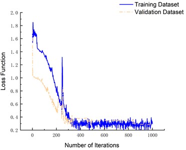
a) With dropout layer
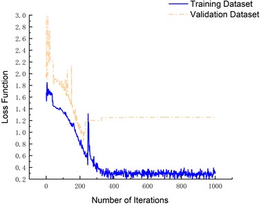
b) No dropout layer
The prediction outcomes for the three-axis errors, namely the -axis, -axis, and -axis, are graphically depicted in Figs. 14, 15, and 16 respectively. A comparative analysis reveals that the WOA-LSTM model yields improved predictions over the LSTM and GRU models. Specifically, concerning the -axis error, the mean root mean square error (RMSE) of the WOA-LSTM model decreases by 49.19 % and 65.98 % relative to the LSTM and GRU models. Similarly, for the -axis error prediction, the WOA-LSTM model achieves a decrease in average RMSE of 23.17 % and 60.82 %, while in predicting the -axis error, the average RMSE drops by 34.63 % and 67.31 %. In order to authenticate the accuracy and robustness of the WOA-LSTM model, an extensive examination of the ball screw error measurement and prediction under a variety of experimental conditions was undertaken. As Table 2 manifests, under equivalent sample sizes, the WOA-LSTM model exhibits notably enhanced prediction accuracy and efficiency vis-à-vis the LSTM and GRU models, with the maximum absolute residuals being 0.0194 mm, 0.0213 mm, and 0.0202 mm for the , , and axes respectively.
Fig. 14Comparison of X-axis three-way error prediction
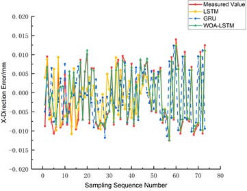
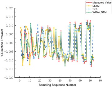
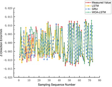
Fig. 15Comparison of Y-axis three-way error prediction
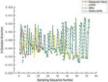
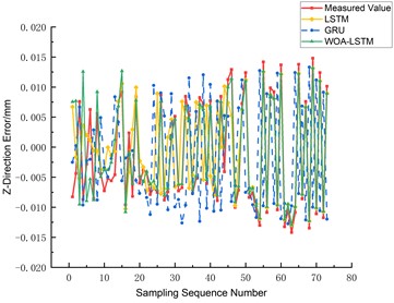
Fig. 16Comparison of Z-axis three-way error prediction
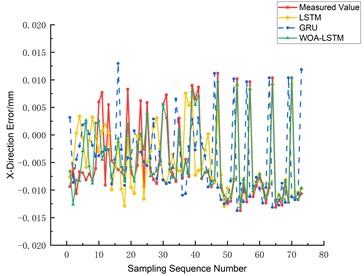
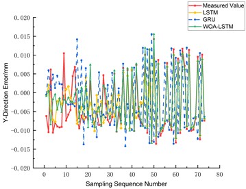
Based on Figs. 14-16, it is evident that the WOA-LSTM model provides the most accurate predictions for the -axis on various axes. Therefore, the prediction is fitted for the -axis. Additionally, Fig. 17 shows that the WOA-LSTM model has a higher R-squared value, indicating a more significant and statistically relevant fitting effect compared to the LSTM model.
Fig. 17Fitting impact of the X-axis forecasts
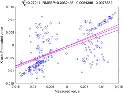
a) LSTM
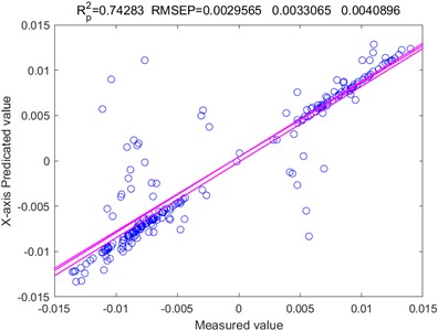
b) WOA-LSTM
Additionally, considering the superior prediction performance on the -axis, the KDE method was employed to fit the error distribution based on the -axis data. Fig. 18 shows that the normalized average width of the prediction intervals becomes narrower with the change in sample data. However, at peak and valley error values, these intervals widen considerably, possibly due to the influence of uncertainty factors on the error data at these extremes.
In an effort to appraise the efficacy of model interval prediction, this paper incorporates two key evaluation indices: Prediction Interval Coverage Probability (PICP) and Normalized Prediction Interval Average Width (PINAW), with their respective calculation formulas given below:
Fig. 18X-axis interval forecasting effectiveness
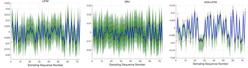
a)-direction
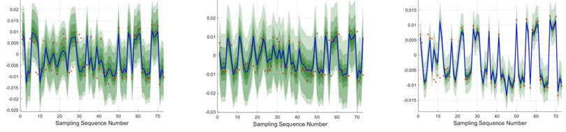
b)-direction
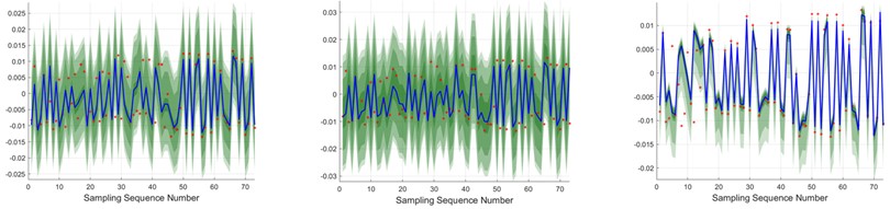
c)-direction

Table 3 consolidates the findings related to the -axis prediction interval coverage (PICP) and normalized prediction interval average width (PINAW) for the three models across varied confidence levels.
The PINAW values of the WOA-LSTM model show a decrease between 53.81 % to 73.56 % compared to the LSTM and GRU models at the 95% confidence level. This trend continues at 90 %, 75 %, and 50 % confidence levels, where the WOA-LSTM model consistently outperforms the other models in both metrics.
To summarize, the WOA-LSTM model not only improves prediction accuracy but also significantly reduces the width of the prediction interval, indicating its superior predictive capabilities. This highlights the significant impact of the Whale Optimization Algorithm (WOA) in optimizing the LSTM model, making the WOA-LSTM model the best choice for precise and efficient prediction of the three-axis screw errors.
Table 3Comparative evaluation of interval estimates under different levels of confidence
Confidence level | Model | PICP (%) | PINAW |
, , | , , | ||
95 % | LSTM | 93.15 %, 87.67 %, 93.15 % | 0.9498, 0.9958, 1.1712 |
GRU | 93.15 %, 90.41 %, 86.30 % | 1.4428, 1.3645, 1.5889 | |
WOA-LSTM | 93.15 %, 93.15 %, 93.15 % | 0.4387, 0.4508, 0.4201 | |
90 % | LSTM | 87.67 %, 84.93 %, 86.30 % | 0.8172, 0.8066, 1.0228 |
GRU | 90.41 %, 83.56 %, 80.82 % | 1.2759, 0.9862, 1.4157 | |
WOA-LSTM | 89.04 %, 87.67 %, 90.41 % | 0.3077, 0.1996, 0.2922 | |
75 % | LSTM | 71.23 %, 73.97 %, 73.97 % | 0.5424, 0.3881, 0.6709 |
GRU | 72.60 %, 75.34 %, 69.86 % | 0.9222, 0.4608, 0.9873 | |
WOA-LSTM | 72.60 %, 79.45 %, 76.71 % | 0.0873, 0.0941, 0.1028 | |
50 % | LSTM | 47.95 %, 54.79 %, 52.05 % | 0.1634, 0.1916, 0.1540 |
GRU | 52.05 %, 49.31 %, 50.68 % | 0.5173, 0.2582, 0.4302 | |
WOA-LSTM | 49.31 %, 49.31 %, 49.32 % | 0.0573, 0.0650, 0.0690 |
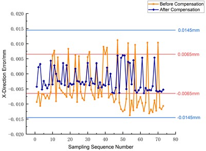
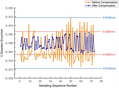
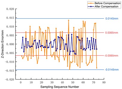
4.2. Experimental verification of error compensation
The -axis of the S7H composite machining center was studied to compensate for machining errors. The three-way error of the -axis before and after the compensation was compared. As shown in Fig. 19, the maximum error of the three-way error of the -axis was significantly reduced from ±0.0145 mm to ±0.006 mm after the compensation. At the same time, the average three-way error was also significantly improved from –0.00486, –0.00325, –0.00209 to –0.00197, –0.00049, –0.00038, –0.00197, –0.00049, –0.00038, and –0.00209, respectively. This means that the average three-way error was improved from –0.00209 to –0.00197, –0.00049 and -0.00038 after the compensation.
Fig. 19Comparison of three-way error before and after compensation
5. Conclusions
The objective of this study is to investigate the implications of dual-end constraints on the precision of ball screw calibration during error compensation procedures and to propose a comprehensive approach for screw error mitigation. Focusing on the feed screws of the axes within the S7H composite machining center, the following salient points emerge from the conducted research:
1) This investigation employs the Whale Optimization Algorithm (WOA) to fine-tune the hyperparameters of the Long Short-Term Memory (LSTM) model, thereby addressing the issues surrounding substantial computational overhead and low search efficiency typically associated with the adjustment of hyperparameters in the three-axis error prediction model for screws.
2) Comparative analysis of the three modeling techniques vis-à-vis experimental measurements of screw errors reveals that the three-axis error prediction model constructed by integrating the WOA with the LSTM neural network demonstrates superior fitting performance. This validates the efficacy of the proposed screw's three-axis error prediction model in accurately forecasting the actual screw errors and enhancing the machining precision of the machine tool.
3) Using QT software and Matlab software for the secondary development of the CNC system, the ball screw error compensation module communicates more effectively with the interpolator to achieve real-time 3-axis error compensation.
4) The empirical outcomes highlight that the radial screw error exerts a significantly greater influence on the machine's practical machining accuracy relative to the axial screw error. Thus, an all-encompassing screw error compensation methodology is devised to cater to different mounting configurations. The effectiveness of this holistic approach is corroborated through error compensation machining experiments, demonstrating an improvement in machining accuracy by approximately 59 %.
References
-
Liu K. et al., “Review on thermal error compensation for feed axes of CNC machine tools,” (in Chinese), Journal of Mechanical Engineering, Vol. 57, No. 3, p. 156, Jan. 2021, https://doi.org/10.3901/jme.2021.03.156
-
R. Ramesh, M. A. Mannan, and A. N. Poo, “Error compensation in machine tools – a review,” International Journal of Machine Tools and Manufacture, Vol. 40, No. 9, pp. 1235–1256, Jul. 2000, https://doi.org/10.1016/s0890-6955(00)00009-2
-
Li T. J., “Study on thermal characterstics and error compensation control method of the ball screw feed drive system for CNC machine tools,” (in Chinese), Northeastern University of China, 2018.
-
Y. Li, W. Zhao, S. Lan, J. Ni, W. Wu, and B. Lu, “A review on spindle thermal error compensation in machine Tools,” International Journal of Machine Tools and Manufacture, Vol. 95, pp. 20–38, Aug. 2015, https://doi.org/10.1016/j.ijmachtools.2015.04.008
-
Li B., Zhang Y., Wang L. P., and Li X. K., “Modeling for CNC machine tool thermal error based on genetic algorithm optimization wavelet neural networks,” (in Chinese), Journal of Mechanical Engineering, Vol. 55, No. 21, pp. 215–220, 2019, https://doi.org/10.3901/jme.2019.21.215
-
P.-L. Liu, Z.-C. Du, H.-M. Li, M. Deng, X.-B. Feng, and J.-G. Yang, “Thermal error modeling based on bilstm deep learning for CNC machine tool,” Advances in Manufacturing, Vol. 9, No. 2, pp. 235–249, Feb. 2021, https://doi.org/10.1007/s40436-020-00342-x
-
H. Shi, Y. Xiao, X. Mei, T. Tao, and H. Wang, “Thermal error modeling of machine tool based on dimensional error of machined parts in automatic production line,” ISA Transactions, Vol. 135, pp. 575–584, Apr. 2023, https://doi.org/10.1016/j.isatra.2022.09.043
-
G. Qianjian and Y. Jianguo, “Application of projection pursuit regression to thermal error modeling of a CNC machine tool,” The International Journal of Advanced Manufacturing Technology, Vol. 55, No. 5-8, pp. 623–629, Dec. 2010, https://doi.org/10.1007/s00170-010-3114-4
-
G. B. Li, D. Gao, Y. Lu, H. Ping, and Y. Y. Zhou, “Adaptive Kalman filter and PSO-GA-BP algorithm for robot error compensation,” (in Chinese), China Mechanical Engineering, Vol. 34, No. 20, pp. 2456–2465, Oct. 2023, https://doi.org/10.3969/j.issn.1004-132x.2023.20.008
-
B. Li, X. Tian, and M. Zhang, “Thermal error modeling of machine tool spindle based on the improved algorithm optimized BP neural network,” The International Journal of Advanced Manufacturing Technology, Vol. 105, No. 1-4, pp. 1497–1505, Sep. 2019, https://doi.org/10.1007/s00170-019-04375-w
-
S.-S. Li, Y. Shen, and Q. He, “Study of the thermal influence on the dynamic characteristics of the motorized spindle system,” Advances in Manufacturing, Vol. 4, No. 4, pp. 355–362, Nov. 2016, https://doi.org/10.1007/s40436-016-0158-1
-
Li Y., Chen G. H., Xia M., and Li B., “Design and simulation optimization of motorized spindle cooling system,” (in Chinese), Chinese Journal of Engineering Design, Vol. 30, No. 1, pp. 39–47, 2023, https://doi.org/10.3785/j.issn.1006-754x.2023.00.008
-
H. Qu, Y. Dai, G. Wang, W.-J. Wen, and C.-F. Xiang, “A review based on the control method of thermal error for high-speedmotorized spindles,” Recent Patents on Engineering, Vol. 17, No. 3, pp. 58–71, May 2022, https://doi.org/10.2174/1872212116666220513114154
-
C. W. Lu, B. Z. Qian, H. M. Wang, and S. T. Xiang, “Key geometric error analysis and compensation method of five-axis cnc machine tools under workpiece feature decomposition,” (in Chinese), China Mechanical Engineering, Vol. 33, No. 14, pp. 1646–1653, 2022, https://doi.org/10.3969/ji.ssn.1004-132x.2022.14.002
-
T. Li, F. Li, Y. Jiang, and H. Wang, “Thermal error modeling and compensation of a heavy gantry-type machine tool and its verification in machining,” The International Journal of Advanced Manufacturing Technology, Vol. 92, No. 9-12, pp. 3073–3092, Apr. 2017, https://doi.org/10.1007/s00170-017-0353-7
-
G. Chen et al., “Modeling method of CNC tooling volumetric error under consideration of Abbé error,” The International Journal of Advanced Manufacturing Technology, Vol. 119, No. 11-12, pp. 7875–7887, Jan. 2022, https://doi.org/10.1007/s00170-021-08494-1
-
C.-W. Wu, C.-H. Tang, C.-F. Chang, and Y.-S. Shiao, “Thermal error compensation method for machine center,” The International Journal of Advanced Manufacturing Technology, Vol. 59, No. 5-8, pp. 681–689, Aug. 2011, https://doi.org/10.1007/s00170-011-3533-x
-
J. Xu, L. Guo, J. Jiang, B. Ge, and M. Li, “A deep learning methodology for automatic extraction and discovery of technical intelligence,” Technological Forecasting and Social Change, Vol. 146, pp. 339–351, Sep. 2019, https://doi.org/10.1016/j.techfore.2019.06.004
-
S. Hochreiter and J. Schmidhuber, “Long short-term memory,” Neural Computation, Vol. 9, No. 8, pp. 1735–1780, Nov. 1997, https://doi.org/10.1162/neco.1997.9.8.1735
-
Y. Y. Guo et al., “Seismic response prediction of electrical equipment interconnected system of traction station based on LSTM neural network,” (in Chinese), Journal of Railway Science and Engineering, Vol. 20, No. 12, pp. 1–11, 2023, https://doi.org/10.19713/j.cnki.43-1423/u.t20231072
-
Xavier Glorot and Yoshua Bengio, “Understanding the difficulty of training deep feedforward neural networks,” Journal of Machine Learning Research, Vol. 9, pp. 249–256, Mar. 2010.
-
D. P. Kingma and J. Ba, “Adam: a method for stochastic optimization,” arXiv:1412.6980, Jan. 2014.
-
“Test code for machine tools-Part 3: Determination of thermal effects,” IS0 230-3, Switzerland, TC 39, 2020.
-
P. Roztocki et al., “Phase recovery and stability: arbitrary phase access for stable fiber interferometers (Laser Photonics Rev. 15(7)/2021),” Laser and Photonics Reviews, Vol. 15, No. 7, Jul. 2021, https://doi.org/10.1002/lpor.202170041
-
I. V. Herasymenko, I. O. Zaitsev, V. I. Latenko, R. D. Myronov, I. A. Ornatsky, and S. O. Fil, “Improving the algorithm for calculating the temperature of the quasilinear resistance sensor PT100,” Tekhnichna Elektrodynamika, Vol. 2023, No. 2, pp. 83–91, Feb. 2023, https://doi.org/10.15407/techned2023.02.083
About this article

This work was supported by Hubei Provincial Natural Science Foundation Joint Fund for Innovation and Development Project (No.: 2022CFD081), Major Science and Technology Projects of Hubei Province (No.: 2021AAA003), Hubei Province Intellectual Property Application Demonstration Project in 2020 and Special Project for Supporting Technological Innovation and Development of Enterprises (No.: 2021BAB011), XiangYang Science and Technology Project in 2022 (No.: 2022ABH006436).
The datasets generated during and/or analyzed during the current study are available from the corresponding author on reasonable request.
Bo Zhou: conceptualization, methodology, software, investigation, data curation, writing-original draft. Guo Hua Chen: methodology, investigation, resources, data curation, writing-review and editing, project administration. Jie Mao: validation, formal analysis, resources. Yi Li: resources, visualization. Shuai Wei Zhang: investigation, data curation.
The authors declare that they have no conflict of interest.
