A simple harmonic quantum oscillator: fractionalization and solution

Batiha, Iqbal M.; Jebril, Iqbal H.; Al-Nana, Abeer A.; Alshorm, Shameseddin

doi:10.21595/mme.2024.23904

Mathematical Models in Engineering

Browse Journal

Submit article

Published: 02 March 2024

Check for updates

A simple harmonic quantum oscillator: fractionalization and solution

Iqbal M. Batiha¹

Iqbal H. Jebril²

Abeer A. Al-Nana³

Shameseddin Alshorm⁴

¹Nonlinear Dynamics Research Center (NDRC), Ajman University, Ajman, 346, United Arab Emirates

^{1, 2, 4}Department of Mathematics, Al Zaytoonah University of Jordan, Amman, 11733, Jordan

³Department of Mathematics, Prince Sattam Bin Abdulaziz University, Alkharj, 11942, Saudi Arabia

Corresponding Author:

Iqbal M. Batiha

Cite the article Download PDF

Abstract

A quantum mechanical system that mimics the behavior of a classical harmonic oscillator in the quantum domain is called a simple harmonic quantum oscillator. The time-independent Schrödinger equation describes the quantum harmonic oscillator, and its eigenstates are quantized energy values that correspond to various energy levels. In this work, we first fractionalize the time-independent Schrödinger equation, and then we solve the generated problem with the use of the Adomian decomposition approach. It has been shown that fractional quantum harmonic oscillators can be handled effectively using the proposed approach, and their behavior can then be better understood. The effectiveness of the method is validated by a number of numerical comparisons.

$A simple harmonic quantum oscillator: fractionalization and solution$

Highlights

Fractionalizing the time-independent Schrödinger equation using Caputo fractional differentiator.
Solving the fractional-order Schrödinger equation with the use of the Adomian decomposition approach.
The effectiveness of the Adomian decomposition approach is validated by a number of numerical comparisons.

1. Introduction

In recent years, fractional calculus – a branch of classical calculus that deals with instructions on non-integer integration and differentiation – has become a fascinating area of study. The notion of fractional operators, which emerged nearly concurrently with their classical equivalents, has garnered considerable attention owing to their multifarious applicability across multiple fields of mathematics and science. It has been demonstrated that fractional differential equations are effective instruments for understanding and simulating intricate engineering, chemical, and physical processes [1-5].

The Schrödinger equation is a key tool in the field of quantum mechanics for explaining how quantum systems behave. This equation, which was created by Erwin Schrödinger in 1926, uses time as an independent variable to describe quantum systems. Time-independent Schrödinger equations (TISE) and time-dependent Schrödinger equations (TDSE) are the two categories into which Schrödinger wave equations fall [5, 6].

Numerous authors have offered both analytical and numerical solutions for TISE and TDSE. The Schrödinger issue has been solved using modern analytical techniques such the Elzaki decomposition methodology, homotopy perturbation, and Adomian decomposition methods. On the other hand, techniques such as the Numerov algorithm for harmonic and linear potentials have been used to produce approximative numerical solutions.

In this work, we study the semi-analytical solution of the Adomian decomposition approach for time-independent Schrödinger equations. The ADM provides an accurate solution and is well-known for its effectiveness in solving Sturm-Liouville issues, ordinary and partial differential equations, nonlinear and stochastic problems, and more. When compared to other approaches, the ADM solves the TISE more quickly and accurately while still offering a series solution [7-10].

The structure of this article is as follows: In part 2, we establish the notations and present the essential concepts, including the fractional operators of the Riemann-Liouville integral and derivative, and the Caputo derivative, which will be utilized throughout this essay. Section 3, employs the ADM to solve the Schrödinger equation for the simple fractional harmonic oscillator, converting it into a Hermite differential equation. In Section 4, we depict some numerical comparisons between the ADM’s solution and the solution reported in some references. Finally, Section 5 summarizes the conclusion of this work.

2. Preliminaries and notion

In this section, we go over the basic ideas of fractional calculus in detail, which forms the basis of our investigation. We also explore the properties of certain operators that are important to our work [11-14].

Definition 2.1. The Riemann-Liouville fractional integral of $f$ of order $γ$ , where $t > 0$ , $n - 1 < γ \leq n$ , $n \in N$ , of a function $f (t)$ is given as follows:

1

I^{γ} f (t) = \frac{1}{Γ (γ)} \int_{0}^{t} (t - τ)^{γ - 1} f (τ) d τ .

The following features of the Riemann-Liouville integral are worth noting:

2

I^{0} f (t) = f (t),

3

I^{γ} t^{m} = \frac{Γ (m + 1)}{Γ (m + γ + 1)} t^{m + γ}, m \geq - 1,

4

I^{γ} I^{B} f (t) = I^{B} I^{γ} f (t), γ, B \geq 0,

5

I^{γ} I^{B} f (t) = I^{γ + B} f (t), γ, B \geq 0 .

Definition 2.2. Let $n - 1 < γ < n$ , such that $n$ is positive integer and $γ \in R^{+}$ , the Riemann Liouville derivative of fractional of order $γ$ is given as follows:

6

D^{γ} f (t) = \frac{1}{Γ (n - γ)} \frac{d^{n}}{d t^{n}} \int_{0}^{t} \frac{f^{(n)} (τ)}{(t - τ)^{γ + 1 - n}} d τ .

Definition 2.3. Suppose that $γ > 0$ , $t > γ$ , $t \in R$ . The Caputo fractional differential operator of order $γ$ , is given as:

7

D^{γ} f (x) = \{\begin{matrix} \frac{1}{Γ (n - γ)} \int_{0}^{t} \frac{f^{(n)} (τ)}{(t - τ)^{γ + 1 - n}} d τ, n - 1 < γ < n \in N, \\ \frac{d^{n}}{d t^{n}} f (t), γ = n \in N . \end{matrix}

Remarks. The Caputo fractional derivative meets the following properties:

1. The power rule property, i.e.:

8

D^{γ} t^{ε} = \{\begin{array}{l} \frac{Γ (ε + 1)}{Γ (ε - γ + 1)} t^{ε - γ} = D^{γ} t^{ε}, & n - 1 < α < n, ε > n - 1, ε \in R, \\ 0, & n - 1 < α < n, ε \leq n - 1, ε \in N . \end{array}

2. The constant property, i.e.:

9

D^{γ} c = 0 .

3. The interpolation property, i.e.:

10

\lim_{γ \to n} D^{γ} f (t) = D^{n} f (t) .

4. The linearity property, i.e.:

11

D^{γ} (λ f (t) + ψ g (t)) = λ D^{γ} f (t) + D^{γ} g (t) ψ .

5. The non-commutation property, i.e.:

12

D^{γ} D^{Ɣ} f (t) = D^{γ + Ɣ} f (t) \neq D^{Ɣ} D^{γ} f (t) .

3. Theory

One typical method for modeling systems with viscoelasticity in damping terms is to incorporate fractional derivatives to introduce memory effects in the system. The mathematical framework offered by fractional calculus makes it possible to include memory effects and produce a more realistic depiction of the behavior of the system.

The damping term in the differential equation can be written as a fractional derivative of the displacement or velocity variable when modeling viscoelasticity damping with fractional derivatives. The memory effects in the damping system are captured by this fractional derivative, enabling a more accurate depiction of the system’s reaction to outside influences.

The core of this study is covered in this section, where we introduce our unique method for solving the Schrödinger equation for the basic fractional harmonic oscillator. In order to do this, we make use of the ADM, a reliable numerical technique that is well-known for its accuracy and efficiency in solving differential equations. Our objective is to transform the original Schrödinger equation into the Hermite differential equation, which is a more manageable form and has fractional order derivatives [15-17].

An important model for studying quantum systems with fractional characteristics is the simple fractional harmonic oscillator. Our goal is to achieve precise answers by utilizing the ADM, which will provide insight into the fascinating occurrences seen in the equation under consideration. The ADM is a perfect fit for this study because of its adaptability in handling nonlinearity and the complexities of fractional calculus [18-20].

In this context, the expression for the time-dependent Schrodinger's equation for a basic fractional harmonic oscillator is:

13

\frac{- h^{2}}{2 r} \frac{d^{2 α} ϕ (x)}{d x^{2 α}} + \frac{1}{2} k x^{2} ϕ (x) = T ϕ (x),

where $h$ , $r$ are constants, $T$ is the energy. It should be observed here that the above model corresponds to inertia terms in the second-order mechanistic counterpart model when alpha = 1. In tha same regard, we should also note that since we are dealing with a physical problem, we will not be considering the positive exponent solution that diverges at. It was noted, meanwhile, that Eq. (13) can be changed to the following form:

14

\frac{d^{2 α} U}{d γ^{2}} - 2 γ \frac{d U}{d γ} + 2 (\frac{T}{h ω} - \frac{1}{2}) U = 0,

where $ϕ (γ) = U (γ) e^{- (γ^{2} / 2)}$ . Now define $λ = (\frac{T}{h ω} - \frac{1}{2})$ and replace the dummy $γ$ with $x$ . This reduces Eq. (14) to the form shown below:

15

D^{2 α} U - 2 x D^{α} U + 2 λ U = 0,

where $U (0) = c_{0}$ , ${D^{α} U}^{'} (0) = c_{1} .$

The ADM is used to tackle this problem, by considering the following form:

16

D^{2 α} U = 2 x D^{α} U - 2 λ U .

Operating $J^{α}$ to both sides of Eq. (16) yields:

D^{α} U - {D^{α} U}^{'} (0) = J^{α} (2 x D^{α} U) - 2 λ J^{α} U,

or:

17

D^{α} U = c_{1} + 2 J^{α} (x D^{α} U) - 2 λ J^{α} U .

Again, by taking $J^{α}$ to both sides of Eq. (17), we obtain:

U - U (0) = J^{α} c_{1} + {2 J}^{2 α} (x D^{α} U) - 2 λ J^{2 α} U .

The result is as follows:

18

U = c_{0} + c_{1} \frac{x^{α}}{Γ (α + 1)} + {2 J}^{2 α} (x D^{α} U) - 2 λ J^{2 α} U,

where $c_{0}$ and $c_{1}$ are arbitrary constants. Following the ADM sense leads to the general solution for $U$ , which would be as:

19

U = \sum_{n = 0}^{\infty} U_{n},

where:

20

U_{0} = c_{0} + c_{1} \frac{x^{α}}{Γ (α + 1)}, U_{n + 1} = {2 J}^{2 α} (x D^{α} U_{n}) - 2 λ J^{2 α} U_{n}, n \geq 0 .

We will show some of the major calculations used above. The following steps show how we calculate $U_{1}$ up to $U_{5}$ . In this regard, we can find:

U_{1} = {2 J}^{2 α} (x D^{α} U_{0}) - 2 λ J^{2 α} U_{0},

which means:

U_{1} = {2 J}^{2 α} (x D^{α} (c_{0} + c_{1} \frac{x^{α}}{Γ (α + 1)})) - 2 λ J^{2 α} (c_{0} + c_{1} \frac{x^{α}}{Γ (α + 1)}),

or:

U_{1} = (\frac{- 2 λ x^{2 α}}{Γ (2 α + 1)}) c_{0} + (\frac{2 x^{2 α + 1}}{Γ (2 α + 2)} - \frac{2 λ x^{3 α}}{Γ (3 α + 1)}) c_{1} .

The next term can be written as:

U_{2} = 2 J^{2 α} (x D^{α} U_{1}) - 2 λ J^{2 α} {(U}_{1}) .

In other words, we have:

U_{2} = - 2^{2} λ c_{0} (\frac{Γ (α + 2) x^{3 α + 1}}{Γ (α + 1) Γ (3 α + 2)} - \frac{x^{4 α}}{Γ (4 α + 1)}) + 2^{2} c_{1} (\frac{Γ (α + 3) x^{3 α + 2}}{Γ (α + 2) Γ (3 α + 3)} - λ \frac{x^{4 α}}{Γ (4 α + 2)} (1 + \frac{Γ (2 α + 2)}{Γ (2 α + 1)}) + \frac{λ^{2} x^{5 α}}{Γ (5 α + 1)}) .

Once more, the next term can be written as:

U_{3} = 2 J^{2 α} (x D^{α} U_{2}) - 2 λ J^{2 α} {(U}_{2}) .

This is equivalent to the following assertion:

U_{3} = - 2^{3} c_{0} (\frac{λ Γ (α + 2) {Γ (2 α + 3) x}^{4 α + 2}}{Γ (α + 1) Γ (2 α + 2) Γ (4 α + 3)} + {λ^{2} x}^{5 α + 1} (\frac{Γ (3 α + 2)}{Γ (3 α + 1) Γ (5 α + 2)} + \frac{Γ (α + 2)}{Γ (α + 1) Γ (5 α + 2)}) - \frac{λ^{3} x^{6 α}}{Γ (6 α + 1)}) + 2^{3} c_{1} (\frac{Γ (α + 3) Γ (2 α + 4) x^{3 α + 2}}{Γ (α + 2) Γ (2 α + 3) Γ (4 α + 4)} - {λ^{2} x}^{5 α + 2} (\frac{Γ (3 α + 3)}{Γ (3 α + 2) Γ (5 α + 3)} (1 + \frac{Γ (2 α + 2)}{Γ (2 α + 1)}) + \frac{Γ (α + 3)}{Γ (α + 2) Γ (5 α + 3)}) + \frac{λ^{2} x^{6 α + 1}}{Γ (6 α + 2)} (\frac{Γ (4 α + 2)}{Γ (4 α + 1)} - (1 + \frac{Γ (2 α + 2)}{Γ (2 α + 1)})) - \frac{λ^{3} x^{7 α}}{Γ (7 α + 1)}) .

Similarly, we can have:

U_{4} = 2 J^{2 α} (x D^{α} U_{3}) - 2 λ J^{2 α} {(U}_{3}),

which consequently gives:

21

U_{4} = \frac{- 2^{4} {λ c}_{0} Γ (α + 2) {Γ (2 α + 3) Γ (3 α + 4) x}^{5 α + 3}}{Γ (α + 1) Γ (2 α + 2) Γ (3 α + 3) Γ (5 α + 4)} + 2^{4} c_{1} \frac{Γ (α + 3) {Γ (2 α + 4) Γ (3 α + 5) x}^{5 α + 4}}{Γ (α + 2) Γ (2 α + 3) Γ (3 α + 4) Γ (5 α + 5)} + \frac{2^{4} λ^{2} c_{0} x^{6 α + 2}}{Γ (6 α + 3)} ((\frac{Γ (α + 2)}{Γ (α + 1)} (\frac{Γ (4 α + 3)}{Γ (4 α + 2)} + \frac{Γ (2 α + 3)}{Γ (2 α + 2)})) + \frac{Γ (3 α + 2) Γ (4 α + 3)}{Γ (3 α + 1) Γ (4 α + 2)}) - \frac{2^{4} λ c_{1} x^{6 α + 3}}{Γ (6 α + 4)} ((1 + \frac{Γ (2 α + 2)}{Γ (2 α + 1)}) \frac{Γ (3 α + 3) Γ (4 α + 4)}{Γ (4 α + 3) Γ (3 α + 2)} + \frac{Γ (α + 3) Γ (4 α + 4)}{Γ (α + 2) Γ (4 α + 3)} + \frac{Γ (α + 3) Γ (2 α + 4)}{Γ (2 α + 3) Γ (α + 2)}) - \frac{2^{4} λ^{3} c_{0} x^{7 α + 1}}{Γ (7 α + 2)} (\frac{Γ (5 α + 2)}{Γ (5 α + 1)} + \frac{Γ (3 α + 2)}{Γ (3 α + 1)} + \frac{Γ (α + 2)}{Γ (α + 1)}) + \frac{2^{4} λ^{2} c_{1} x^{7 α + 2}}{Γ (7 α + 3)} ((1 + \frac{Γ (2 α + 2)}{Γ (2 α + 1)}) (\frac{Γ (3 α + 3)}{Γ (3 α + 2)} + \frac{Γ (5 α + 3)}{Γ (5 α + 2)}) + \frac{Γ (α + 3)}{Γ (α + 2)} + \frac{Γ (4 α + 2) Γ (5 α + 3)}{Γ (4 α + 1) Γ (5 α + 2)}) + \frac{2^{4} λ^{4} c_{0} x^{8 α}}{Γ (8 α + 1)} + \frac{2^{4} λ^{3} c_{1} x^{8 α + 1}}{Γ (8 α + 2)} ((1 + \frac{Γ (2 α + 2)}{Γ (2 α + 1)}) + \frac{Γ (4 α + 2)}{Γ (4 α + 1)} + \frac{Γ (6 α + 2)}{Γ (6 α + 1)}) + \frac{2^{4} λ^{4} c_{1} x^{9 α}}{Γ (9 α + 1)} .

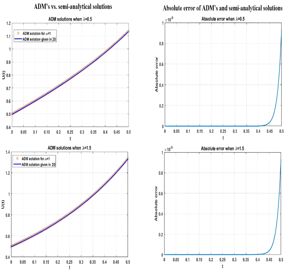
If we continue in this manner, we got the desired solution reported in Eq. (19). To show the validity of our solution, we compare the ADM’s solution with the solution reported in [20] in Fig. 1 and Fig. 2 by taking $α =$ 1 and $λ$ = {0.5, 1.5}. Obviously, we can observe that the proposed solution coincides with the solution we compare, and this confirms the validity of the proposed solution.

Fig. 1ADM’s solution vs. the solution in [20] according to λ= 0.5

Fig. 2ADM’s solution vs. the solution in [20] according to λ= 1.5

Fig. 3Absolute error between the ADM’s solution and the solution in [20]

For more description, we plot in Fig. 3 and Fig. 4, the absolute errors gained from the performance comparison. These figures demonstrate the advantage of the suggested method of fractionalizing the model in question. However, the limitation of our proposed approach lies in the lack of capabilities to obtain a general form of $U_{n}$ that can generate all other components of the desired solution, and this will be left to the future for more consideration.

Fig. 4Absolute error between the ADM’s solution and the solution in [20] when λ= 0.5

4. Conclusions

In this study, a generalized form of the time-independent Schrödinger equation has been successfully proposed in its fractional simple harmonic quantum oscillator. The ADM has been used to obtain a semi-analytical solution for such an oscillator. This solution has proved its validity with an existing solution in [20] when a classical case of the generalized form is taken into consideration.

References

H. Goldstein, C. P. Poole, and J. L. Safko, Classical Mechanics. Boston: Addison Wesley, 2002.

Publisher
T. Hamadneh et al., “General methods to synchronize fractional discrete reaction-diffusion systems applied to the glycolysis model,” Fractal and Fractional, Vol. 7, No. 11, p. 828, Nov. 2023, https://doi.org/10.3390/fractalfract7110828

Publisher
G. B. Arfken and H. Weber, Mathematical Methods for Physicists. San Diego: Academic Press, 2001.

Search CrossRef
J. Biazar, E. Babolian, and R. Islam, “Solution of the system of ordinary differential equations by Adomian decomposition method,” Applied Mathematics and Computation, Vol. 147, No. 3, pp. 713–719, Jan. 2004, https://doi.org/10.1016/s0096-3003(02)00806-8

Publisher
A.-M. Wazwaz, “Approximate solutions to boundary value problems of higher order by the modified decomposition method,” Computers and Mathematics with Applications, Vol. 40, No. 6-7, pp. 679–691, Sep. 2000, https://doi.org/10.1016/s0898-1221(00)00187-5

Publisher
B. Zhang and J. Lu, “Exact solutions of homogeneous partial differential equation by a new Adomian decomposition method,” Procedia Environmental Sciences, Vol. 11, pp. 440–446, Jan. 2011, https://doi.org/10.1016/j.proenv.2011.12.070

Publisher
S. Somali and G. Gokmen, “Adomian decomposition method for nonlinear Sturm-Liouville problems,” Surveys in Mathematics and its Applications, Vol. 2, pp. 11–20, 2007.

Search CrossRef
A. Cheniguel and A. Ayadi, “Solving heat equation by the Adomian decomposition method,” in Proceedings of the World Congress on Engineering, 2011.

Search CrossRef
M. Dehghan, “The use of Adomian decomposition method for solving the one-dimensional parabolic equation with non-local boundary specifications,” International Journal of Computer Mathematics, Vol. 81, No. 1, pp. 25–34, Jun. 2010, https://doi.org/10.1080/0020716031000112321

Publisher
D. N. Khan Marwat and S. Asghar, “Solution of the heat equation with variable properties by two-step Adomian decomposition method,” Mathematical and Computer Modelling, Vol. 48, No. 1-2, pp. 83–90, Jul. 2008, https://doi.org/10.1016/j.mcm.2007.09.003

Publisher
I. G. Rochdi Jebari and A. Boukricha, “Adomian decomposition method for solving nonlinear diffusion equation with convection term,” International Journal of Pure and Applied Sciences and Technology, Vol. 12, pp. 49–58, 2012.

Search CrossRef
F.-K. Yin, W.-Y. Han, and J.-Q. Song, “Modified Laplace decomposition method for Lane-Emden type differential equations,” International Journal of Applied Physics and Mathematics, Vol. 3, No. 2, pp. 98–102, Jan. 2013, https://doi.org/10.7763/ijapm.2013.v3.184

Publisher
F. Mainardi, “Fractional Calculus,” Fractals and Fractional Calculus in Continuum Mechanics, pp. 291–348, Jan. 1997, https://doi.org/10.1007/978-3-7091-2664-6_7

Publisher
Q. Wang, “Homotopy perturbation method for fractional KdV equation,” Applied Mathematics and Computation, Vol. 190, No. 2, pp. 1795–1802, Jul. 2007, https://doi.org/10.1016/j.amc.2007.02.065

Publisher
R. L. Burden and J. D. Faires, Numerical Analysis. Pacific Grove: Brooks/Cole, 2011.

Search CrossRef
R. Courant, Methods of Mathematical Physics, Volume II: Partial Differential Equations. New York: Inter science Publishers Inc., 1966.

Search CrossRef
R. I. Nuruddeen, “Elzaki decomposition method and its applications in solving linear and nonlinear Schrodinger equations,” Sohag Journal of Mathematics, Vol. 4, No. 2, pp. 31–35, May 2017, https://doi.org/10.18576/sjm/040201

Publisher
J. Biazar, R. Ansari, K. Hosseini, and P. Gholamin, “Solution of the linear and nonlinear Schrodinger equations using homotopy perturbation and Adomian decomposition methods,” International Mathematical Forum. Journal for Theory and Applications, Vol. 3, pp. 1891–1897, 2008.

Search CrossRef
A. Sadighi and D. D. Ganji, “Analytic treatment of linear and nonlinear Schrödinger equations: A study with homotopy-perturbation and Adomian decomposition methods,” Physics Letters A, Vol. 372, No. 4, pp. 465–469, Jan. 2008, https://doi.org/10.1016/j.physleta.2007.07.065

Publisher
A. A. Anulo, “On analyzing numerical solution of time independent Schrodinger equation,” Global Scientific Journals, Vol. 7, No. 6, pp. 190–211, 2019.

Search CrossRef
A. K. Jaradat, A. A. Obeidat, M. A. Gharaibeh, and M. K. Hasan Qaseer, “Adomian decomposition approach to solve the simple harmonic quantum oscillator,” International Journal of Applied Engineering Research, Vol. 13, No. 2, pp. 1056–1059, 2018.

Search CrossRef
I. M. Batiha, A. Bataihah, A. A. Al-Nana, S. Alshorm, I. H. Jebril, and A. Zraiqat, “A numerical scheme for dealing with fractional initial value problem,” International Journal of Innovative Computing, Information and Control, Vol. 19, No. 3, pp. 763–774, Jan. 2023, https://doi.org/10.24507/ijicic.19.03.763

Publisher
I. M. Batiha, S. Alshorm, A. Al-Husban, R. Saadeh, G. Gharib, and S. Momani, “The n-point composite fractional formula for approximating Riemann-Liouville integrator,” Symmetry, Vol. 15, No. 4, p. 938, Apr. 2023, https://doi.org/10.3390/sym15040938

Publisher
I. M. Batiha, O. Y. Ababneh, A. A. Al-Nana, W. G. Alshanti, S. Alshorm, and S. Momani, “A numerical implementation of fractional-order PID controllers for autonomous vehicles,” Axioms, Vol. 12, No. 3, p. 306, Mar. 2023, https://doi.org/10.3390/axioms12030306

Publisher
I. M. Batiha, S. Momani, S. Alshorm, and A. Ouannas, “Numerical solutions of stochastic differential equation using modified three-point fractional formula,” in 2023 International Conference on Fractional Differentiation and Its Applications (ICFDA), pp. 1–5, Mar. 2023, https://doi.org/10.1109/icfda58234.2023.10153192

Publisher
I. M. Batiha et al., “Common fixed-point theorem in non-Archimedean menger PM-spaces using CLR property with application to functional equations,” IAENG International Journal of Applied Mathematics, Vol. 53, No. 1, 2023.

Search CrossRef
I. M. Batiha, Z. Chebana, T.-E. Oussaeif, A. Ouannas, S. Alshorm, and A. Zraiqat, “Solvability and dynamics of superlinear reaction diffusion problem with integral condition,” IAENG International Journal of Applied Mathematics, Vol. 53, No. 1, pp. 1–9, 2023.

Search CrossRef
I. M. Batiha, N. Alamarat, S. Alshorm, O. Y. Ababneh, and S. Momani, “Semi-analytical solution to a coupled linear incommensurate system of fractional differential equations,” Nonlinear Functional Analysis and Applications, Vol. 28, No. 2, pp. 449–471, Jun. 2023, https://doi.org/10.22771/nfaa.2023.28.02.09

Publisher
I. M. Batiha, S. Alshorm, I. Jebril, A. Zraiqat, Zaid Momani, and S. Momani, “Modified 5-point fractional formula with Richardson extrapolation,” AIMS Mathematics, Vol. 8, No. 4, pp. 9520–9534, Jan. 2023, https://doi.org/10.3934/math.2023480

Publisher

About this article

Received

29 December 2023

Accepted

17 February 2024

Published

02 March 2024

DOI

https://doi.org/10.21595/mme.2024.23904

Keywords

harmonic oscillator

Adomian decomposition

Hermite polynomial

Acknowledgements

The authors have not disclosed any funding.

Data Availability

The datasets generated during and/or analyzed during the current study are available from the corresponding author on reasonable request.

Author Contributions

Conceptualization, Iqbal M. Batiha; methodology, Iqbal H. Jebril and Abeer A. Al-Nana; validation, Shameseddin Alshorm; formal analysis, Iqbal M. Batiha.; investigation, Iqbal H. Jebril and Abeer A. Al-Nana; resources, Shameseddin Alshorm; data curation, Iqbal M. Batiha; writing-original draft, Abeer A. Al-Nana; visualization, Iqbal H. Jebril; supervision, Iqbal M. Batiha. All authors have read and agreed to the published version of the manuscript.

Conflict of interest

The authors declare that they have no conflict of interest.

This is an open access article distributed under the Creative Commons Attribution License, which permits unrestricted use, distribution, and reproduction in any medium, provided the original work is properly cited.

Previous article in issue Previous Next article in issue Next

Research article

2019 03 15

Adomian’s decomposition method to modeling power functionally graded thermoelastic materials in heat transfer and thermal stress analysis

Hamdy M. Youssef, Eman A. N. Al-Lehaibi

Research article

2018 02 15

Dynamical response of fractional-order nonlinear system with combined parametric and forcing excitation

Hai Jun Xing, Ke Shi Xiao, Peng Sai Song, Lin Ru Li

Research article

2017 12 31

Adaptive mesh refinement method for optimal control based on Hermite-Legendre-Gauss-Lobatto direct transcription

Humin Lei, Tao Liu, Deng Li, Jikun Ye

Research article

2017 11 15

Application of the polynomial dimensional decomposition method in a class of random dynamical systems

Kuan Lu, Lei Hou, Yushu Chen

I. M. Batiha, I. H. Jebril, A. A. Al-Nana, and S. Alshorm, “A simple harmonic quantum oscillator: fractionalization and solution,” Mathematical Models in Engineering, Vol. 10, No. 1, pp. 26–34, Mar. 2024, https://doi.org/10.21595/mme.2024.23904

Copy Extrica

Copied to clipboard!

TY  - JOUR
DO  - 10.21595/mme.2024.23904
UR  - https://doi.org/10.21595/mme.2024.23904
TI  - A simple harmonic quantum oscillator: fractionalization and solution
T2  - Mathematical Models in Engineering
AU  - Batiha, Iqbal M.
AU  - Jebril, Iqbal H.
AU  - Al-Nana, Abeer A.
AU  - Alshorm, Shameseddin
PY  - 2024
DA  - 2024/03/02
PB  - Extrica
SP  - 26-34
VL  - 10
IS  - 1
SN  - 2351-5279
SN  - 2424-4627
ER  - 

Copy Ris

Copied to clipboard!

 @article{Batiha_2024, title={A simple harmonic quantum oscillator: fractionalization and solution}, volume={10}, ISSN={2424-4627}, url={https://doi.org/10.21595/mme.2024.23904}, DOI={10.21595/mme.2024.23904}, number={1}, journal={Mathematical Models in Engineering}, publisher={JVE International Ltd.}, author={Batiha, Iqbal M. and Jebril, Iqbal H. and Al-Nana, Abeer A. and Alshorm, Shameseddin}, year={2024}, month=mar, pages={26–34} }

Copy Bibtex

Copied to clipboard!

[1]I. M. Batiha, I. H. Jebril, A. A. Al-Nana, and S. Alshorm, “A simple harmonic quantum oscillator: fractionalization and solution,” Mathematical Models in Engineering, vol. 10, no. 1, pp. 26–34, Mar. 2024, doi: 10.21595/mme.2024.23904.

Copy IEEE

Copied to clipboard!

Batiha, Iqbal M., Iqbal H. Jebril, Abeer A. Al-Nana, and Shameseddin Alshorm. “A Simple Harmonic Quantum Oscillator: Fractionalization and Solution.” Mathematical Models in Engineering 10, no. 1 (March 2, 2024): 26–34. https://doi.org/10.21595/mme.2024.23904.

Copy Chicago

Copied to clipboard!

A simple harmonic quantum oscillator: fractionalization and solution

Abstract

Highlights

1. Introduction

2. Preliminaries and notion

3. Theory

4. Conclusions

References

About this article

Related Articles