Abstract
The method of electromagnetic signal modulation recognition based on wavelet transform convolutional neural network is studied to improve the effect of electromagnetic signal modulation recognition. By analyzing the electromagnetic signal modulation model, the original electromagnetic signal is preprocessed by wavelet transform to remove the noise of the original electromagnetic signal. The processed electromagnetic signal is used as the input of convolutional neural network, and the electromagnetic signal feature vector is extracted through the convolution layer of convolutional neural network. By using full connection operation, the advanced feature vector of electromagnetic signal is integrated, and the electromagnetic signal is classified by softmax function, and the electromagnetic signal modulation recognition result is output, thus realizing the electromagnetic signal modulation recognition. The experimental results show that when the number of layers of wavelet decomposition is 7 and the wavelet function is Db9, the wavelet transform has the best denoising effect on electromagnetic signal data. At the same time, the network training efficiency of this method is high, and the accuracy of electromagnetic signal modulation recognition is as high as 97.2 %, which improves the effect of electromagnetic signal modulation recognition and is suitable for various types of electromagnetic signal modulation recognition.
Highlights
- By analyzing the mixing model of magnetic semaphore, the original magnetic semaphore is preprocessed by wavelet transform.
- The feature vector of magnetic semaphore is extracted by convolutional layer of convolutional neural network.
- The advanced eigenvector of magnetic semaphore is integrated by full connection operation.
1. Introduction
With the wide use of all kinds of radio equipment, there are more and more radiation targets in the electromagnetic environment, and the electromagnetic spectrum is more and more congested [1]. Electromagnetic signals of different uses overlap in time, space and frequency domain, and often face thousands of electromagnetic targets. Electromagnetic signals are mainly in the form of electromagnetic waves [2], and the electromagnetic signal density is as high as several million pulses per second. Automatic modulation recognition (AMR) is an important technology for demodulating electromagnetic signals [3], which is mainly used in electronic warfare in military affairs and illegal supervision in civil fields. AMR technology can also improve the spectrum efficiency in cognitive radio and software radio, so it is of great academic value and practical significance to study efficient and reliable modulation recognition technology.
The traditional electromagnetic signal modulation recognition method has limited expressive ability when faced with complex signals [4], and it becomes more and more difficult to effectively classify and recognize different emitter targets. In such a complex scene, human understanding ability can neither complete the perception of a large number of data, nor can its understanding speed match the information update speed, thus easily causing a series of problems such as perceptual errors or untimely perception of key targets and situations. At present, the identification methods based on the signal characteristics of electromagnetic signals mainly use manual methods to extract signal characteristics and realize discrimination [5]. Common electromagnetic signal feature extraction methods include time domain analysis [6], frequency domain analysis, instantaneous autocorrelation, spectral correlation and time-frequency domain analysis. These methods generally transform the sampled signal and extract its features [7], and realize signal recognition through the feature vectors with high separability. The selection of classifiers is generally based on machine learning [8], such as K-k-Nearest Neighbor, kNN), support vector machines (SVM) [9], decision tree (DT) and so on. In the past, the manual method of electromagnetic signal modulation recognition needed a lot of time and the recognition efficiency was not high, so relevant scholars began to study the method of electromagnetic signal modulation recognition. For example, Dadgarnia, A. and others put forward an automatic identification method using time domain convolution network [10], which uses time domain convolution network to extract the characteristics of electromagnetic signals and complete the modulation identification of electromagnetic signals. However, this method does not preprocess the electromagnetic signal, and is affected by the noise of the electromagnetic signal, which leads to the low accuracy of extracting the characteristics of the electromagnetic signal. Lei, R. et al. extracted the signal identification method under uniaxial compression [11], which used principal component analysis to extract the characteristics of electromagnetic signals and complete the modulation identification of electromagnetic signals. However, this method has a large amount of calculation in the process of data analysis, which leads to a long time for electromagnetic signal modulation recognition. Ohnishi, A. and others put forward a method based on mode of electromagnetic wave identification [12], which decomposes the electromagnetic signal by modal decomposition, extracts the time-frequency feature vector of the electromagnetic signal, and completes the modulation identification of the electromagnetic signal. However, this method is influenced by the selection of modal parameters, and its ability to extract time-frequency feature vectors of electromagnetic signals is poor. Palm. et al. put forward the electromagnetic signal detection method of beta binomial autoregressive moving average model [13], which constructs beta binomial autoregressive moving average model, and realizes electromagnetic signal modulation recognition through training this model. However, this method takes a long time to train the model, which leads to poor modulation recognition effect of electromagnetic signals. Akilli, M. et al. put forward Duffing's weak periodic electromagnetic signal modulation identification method [14], constructed Duffing model, input the collected electromagnetic signals into Duffing model, and obtained the electromagnetic signal modulation identification result after model training. However, the calculation process of this method is too complicated, which leads to the low efficiency of electromagnetic signal modulation recognition. After years of development, people have made some progress in feature extraction of electromagnetic signals. However, the existing electromagnetic signal features usually need a lot of energy to be extracted by people with relevant professional backgrounds, which is difficult to realize automation and intelligence and cannot meet the needs of large-scale data real-time processing.
Wavelet transform (WT) has a good application effect in the field of signal denoising. By decomposing and processing wavelet at multi-resolution, the interference electromagnetic signals with different frequencies can be separated and the disturbed electromagnetic signals can be attenuated. Convolutional neural networks (CNN) have good robustness, and have been widely used in image recognition, signal recognition, data classification and other fields, and has achieved good application results. Therefore, in view of the limitations of the above methods, wavelet transform and convolutional neural network are combined and applied to electromagnetic signal modulation recognition to improve the accuracy of electromagnetic signal modulation recognition.
2. Electromagnetic signal modulation recognition
2.1. Wavelet transform electromagnetic signal preprocessing
2.1.1. Electromagnetic signal modulation model
Analyzing the electromagnetic signal modulation model [15] is helpful to improve the efficiency of subsequent electromagnetic signal modulation recognition. The modulated electromagnetic signal is usually sampled and stored in the form of IQ (Intelligence Quotient) data, so the received electromagnetic signal can be expressed as:
Among them: and respectively represent the orthogonal component and in-phase component of an electromagnetic signal and a set of sample values, represents a constant.
With the complexity of electronic environment and physical environment, electromagnetic signals are seriously distorted in poor communication environment. There are many kinds of interference noises in the process of electromagnetic signal transmission. In this paper, the noise is divided into additive noise and multiplicative noise according to the relationship between signal and noise, whose expression is:
where, represents white noise in electromagnetic signals; represents electric field intensity. The sampling rate is 8 kHz, the sensitivity is 50 V/m, and the measurement unit is the electric field strength.
Because the modulation recognition accuracy of electromagnetic signals is at a very low level and it is difficult to improve when they are directly recognized under different signal-to-noise ratios. Therefore, empirical mode decomposition and variational mode decomposition methods were not effective in denoising electromagnetic signals in the past [16]. Therefore, wavelet transform will be combined to denoise electromagnetic signals with serious distortion, which will lay the foundation for electromagnetic signal modulation identification of convolutional neural networks and improve the accuracy of electromagnetic signal modulation identification under different signal-to-noise ratios.
2.1.2. Wavelet transform electromagnetic signal denoising processing
Based on the analysis of the electromagnetic signal modulation model, the original electromagnetic signal is decomposed by wavelet transform, and the high-frequency electromagnetic signal with small amplitude and the low-frequency electromagnetic signal with large amplitude can be obtained. Through the mapping of threshold function, a series of wavelet coefficient prediction values are obtained, and these prediction values are used for reconstruction to achieve the purpose of denoising.
The general form of wavelet basis function is as follows:
where: constant can change the scale of the wavelet basis function and change the time-frequency resolution. Constant causes the wavelet basis function to translate in time. In this paper, continuous wavelet transform is used, and the complex Morlet function is selected by wavelet basis. The basic steps are as follows:
(1) The original electromagnetic signal and wavelet basis function performing inner product operation to obtain wavelet coefficients:
The value of is changed in a step of to shift the wavelet base until the coverage of the modulated electromagnetic signal ends.
(3) Changing the wavelet scale , repeat steps (1) and (2) to obtain wavelet coefficients with different resolutions.
The main methods of wavelet denoising threshold selection are fixed threshold, adaptive threshold, heuristic threshold, maximum and minimum threshold. The specific process of threshold selection is that the mother wavelet function can decompose the original electromagnetic signal into n details and profiles , if the threshold of is , then:
where: is a wavelet coefficient without threshold processing; is the truncated value of . From the threshold processing results and the th layer reconstruct the electromagnetic signal, and the denoising result of the electromagnetic signal can be obtained. Set is a scale function of multi-resolution analysis, and its specific expression is as follows:
where: is a scale function; is a real number; is the standard orthogonal basis of multi-resolution analysis; is the scale coefficient. In the construction of wavelet, it is not necessary to know the specific forms of scale function and wavelet function, but only to know we can calculate the wavelet decomposition and recovery.
When processing wavelet packet coefficients, it is easy to produce pseudo-Gibbs phenomenon by using hard threshold function to reduce noise; Soft threshold function is used to reduce noise, which is easy to cause distortion such as edge blur. Therefore, in view of the defects of soft and hard threshold methods, combined with the energy distribution characteristics of wavelet packet coefficients in each frequency band after decomposition, a new threshold function is constructed as follows:
where: is the wavelet coefficient value; is the wavelet coefficient value after the threshold is applied; is any normal number; is the set threshold. The threshold function can be changed by changing value to get any function between soft and hard threshold functions.
In order to improve the denoising effect of electromagnetic signals, wavelet transform needs to construct a two-scale equation of Daubechies wavelet [17], which is specifically expressed as:
Among them: is a wavelet function; is an integer set; is the scale coefficient.
The process of constructing the two-scale equation of Daubechies wavelet is as follows:
Step 1: Select a positive integer that .
Step 2: Select a polynomial with the following expression:
Among them: , is algebraic polynomials with real coefficients; is a real number between [0, 1].
Step 3: Select algebraic polynomials with real coefficients., make, in which:.
Step 4: Take, then , in which: is the maximum value of non-zero data in a two-scale sequence; is Gaussian white noise; is a low-pass filter with linear phase. The smoothness of the Daubechies wavelet increases with the number of decomposition layers .
The specific process of denoising the original electromagnetic signal by wavelet transform is shown in Fig. 1.
Fig. 1Data processing flow of electromagnetic signal denoising based on wavelet transform
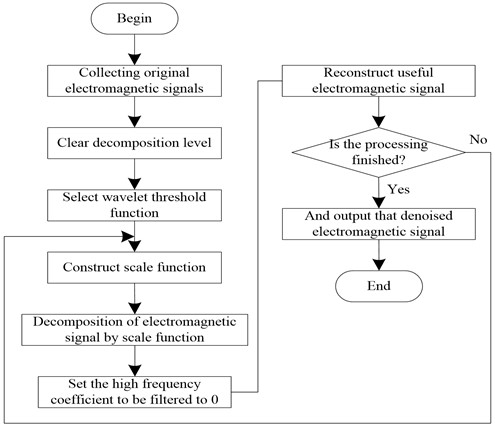
As can be seen from Fig. 1, the data processing flow of electromagnetic signal denoising based on wavelet transform mainly includes three parts: wavelet decomposition, threshold quantization of decomposed high-frequency coefficients and wavelet reconstruction. The analog signals of all channels are collected, and the decomposition levels are determined. At the same time, the scale equation and wavelet threshold are selected as the mother wavelet of electromagnetic signal decomposition. The collected original electromagnetic signals are processed according to the decomposition algorithm, and the high-frequency electromagnetic noise signal coefficients are filtered to obtain useful electromagnetic signals, and these useful electromagnetic signals are reconstructed to obtain the denoised electromagnetic signals. The adaptive threshold selection method can dynamically adjust the threshold according to the local characteristics of the signal to distinguish the noise from the signal more effectively. Sparse representation theory holds that real signals can be represented with fewer non-zero coefficients under certain wavelet bases. Therefore, the signal can be filtered by using the sparsity property of the signal combined with the wavelet transform. For example, an optimization algorithm based on sparse constraints, such as compressed sensing, can be used to improve the filtering effect. The multi-scale decomposition and reconstruction methods are tried to better preserve the information of signals in different frequency ranges.
2.2. Convolution neural network to extract the characteristics of electromagnetic signals
The denoised electromagnetic signal obtained by wavelet transform in section 2.1 is used as the input of convolutional neural network, and the characteristics of electromagnetic signal are extracted by convolutional neural network to complete the modulation recognition of electromagnetic signal.
2.2.1. Convolution extends through the network
Convolution stretching network is a kind of feedforward neural network [18], and the basic network model is generally composed of multiple convolution layers, pooling layers and fully connected layers. The convolution layer acts as a filter, extracting features from input data, and extracting new features by weighted summation of neurons in the upper layer. The calculation formula is as follows:
Among them: represents the input of the convolutional layer of layer , and this paper refers to the eigenvectors carried by electromagnetic signals; represents the offset value of the layer ; represents the weight of the layer .
The activation function layer is usually located after the convolution layer. The extracted linear features are mapped into nonlinear features by activating functions. Among them, the activation function ReLU is widely used in convolutional neural networks. The calculation formula is as follows:
Among them: represents the input of the layer , represents the output obtained by nonlinear mapping of the input by the activation function.
Pool layer is mainly responsible for down sampling. By calculating the nodes in different regions of the feature, the dimension of the nonlinear feature map is reduced. The advantage of this operation method is that it can reduce parameters, reduce computational complexity and prevent over-fitting. The calculation formula is as follows:
Among them: represents the output obtained by maximizing the pool of nonlinear features.
The fully connected layer is to map features to the sample label space and integrate features together. Classify by softmax, express the output as probability, select the maximum probability as the prediction label and output it to complete the classification. The calculation formula is as follows:
Among them: represents a prediction tag, represents the class sample; represents the number of categories.
The training process of convolutional neural network is as follows:
Step 1: Parameter initialization. Before the convolutional neural network starts training, the parameters of each node need to be initialized. The method adopted is to initialize each parameter to a random value close to 0.
Step 2: Parameter updating. Convolutional neural network uses backward propagation gradient descent to make the parameters of each node gradually approach the optimal solution [19]. After the parameters of each node are initialized, the model prediction results are obtained by forward calculation, and the residual of each node in the last layer of the network is calculated according to the predicted values, and then the residual of each node in each layer is calculated reversely from the last layer, so as to obtain the partial derivative of the loss function to the parameters, and then the parameters are updated.
The concrete process of calculating the residual error and updating the parameters of CNN network: The labeled sample data set used for training convolutional neural network is actually a collection of several input-output pairs, and the loss function is used to measure the deviation between the predicted output value and the actual output value of convolutional neural network during training. The smaller the loss function, the better the model performance. Commonly used loss functions include 0-1 loss function, absolute loss function and mean square error loss function. The definition of residual is the loss function to thefloor levelpartial derivatives of the nodes are used to calculate the partial derivatives of the loss function to the parameters. The formula of residual is as follows:
Among them:represents loss function; represents the floor level nodes; represents the residual of the node.
The expression of the residual of each node in the last layer is as follows:
Among them: represents the actual value; represents that derivative of the activation function; represents the floor level nodes; represents the activation value of the last node.
The calculation formula of node residual in other layers is as follows:
Among them: represents the weight of nodes floor level node to node floor level node.
Using the residual of each node, the partial derivative of the loss function to the parameter can be calculated, and the specific solution formula is:
Among them: represents the floor level node offset.
Finally, the update is implemented according to the parameter update, and the parameter update is as follows:
Among them: represent learning rate.
2.2.2. Electromagnetic signal modulation identification process
The electromagnetic signal modulation identification process based on wavelet transform convolutional neural network is as follows:
Step 1: The electromagnetic signal obtained by wavelet transform is used as CNN input.
Step 2: The convolution layer in CNN is used to extract the feature vectors of electromagnetic signals, and the specific process is as follows:
The convolutional neural network used in this paper includes three convolution layers, one fully connected layer and one output layer. The first layer of convolutional neural network adopts one-dimensional convolution layer, which performs convolution operation on one-dimensional feature vector of input denoised electromagnetic signal. After parameter optimization, the convolution kernel with the size of is adopted, the number of filters is set to 64, the step size is set to 1, and 1, Padding is set to same. The convolution kernel gradually slides over the original input data, and the value of the convolution kernel is multiplied by the value of the corresponding position in the input feature vector. Then, a nonlinear activation function ReLU is used to improve the representation ability of the network model. The specific formula is as follows:
Among them: represents the electromagnetic signal to be identified, which carries 100 feature vectors. and respectively represent the weight and offset value of the convolution layer of the first layer, represents the output of the first layer.
The second layer of convolutional neural network adopts one-dimensional convolution layer, and performs convolution operation on the output electromagnetic signal feature vector of the first layer again. The convolution kernel is adopted, and the number of filters is set to 256, the step size is set to 2, and the 2, Padding is set to same, which gradually slides over the input data. Similarly, its value is multiplied by the value of the corresponding position, and then the output of the second layer is obtained through a nonlinear activation function ReLU [20]. The specific formula is as follows:
Among them: represents the input of the second layer, and respectively represents the weight and offset value of the convolution layer of the second layer, represents the output of the second layer.
The third layer of convolutional neural network adopts one-dimensional convolution layer, and the output electromagnetic signal feature vector of the second layer is analyzed perform another convolution operation. Using a convolution kernel of 13, the number of filters is set to 512, the step size is set to 2, padding is set to the same. Gradually slide over the input, multiply its value with the corresponding position, and then get the output of the third layer through a nonlinear activation function ReLU. The specific formula is as follows:
Among them: represents the input of the third layer, and respectively represent the weight and offset value of the convolution layer of the third layer, represents the output of the third layer. So far, the electromagnetic signal to be identified has undergone three one-dimensional convolution operations to get 512 features after mapping.
Thirdly, the modulation mode of electromagnetic signal is accurately identified by combining the full connection layer softmax classifier of convolutional neural network.
The fourth layer of convolutional neural network adopts a fully connected layer. First, all the feature maps output by the third layer of convolutional neural network are integrated into a vector, which is used as the input of fully connected layer. After the full connection operation of 128 neurons, the features extracted from the convolution layer are integrated to obtain higher-level features, which lays the foundation for subsequent recognition. The specific formula is as follows:
Among them: represents the input of the fourth layer, and respectively represent the weight and offset value of the fourth convolution layer, represents the output of the fourth layer. So far, the electromagnetic signal to be identified has been mapped to 256 features through the full connection layer.
The fifth layer of convolutional neural network is the output layer, and the final classification is realized by full connection operation. The softmax function is selected here, which can map the output of neurons to the probability space and obtain the probability of the modulation type of the electromagnetic signal to be measured. The formula is as follows:
Among them: and respectively represent the weight and offset value of the fourth convolution layer, represents a prediction tag, represents the output of the fully connected layer, represents the actual electromagnetic signal type, represents the predicted electromagnetic signal type.
Through the above steps, the modulation recognition of electromagnetic signals is realized.
3. Experimental analysis and results
In order to verify the application effect of the method in this paper, Radio ML2016.10a data set is used as input data in the experiment, which is often used in the research of electromagnetic signal modulation recognition at present. The data set contains six types of electromagnetic signals, namely binary phase shift keying (BPSK), quadrature phase shift keying (QPSK), 8 Phase Shift Keying, (8PSK), 16 quadrature amplitude modulation, (16QAM), 64-bit quadrature amplitude modulation (64 QAM), and binary frequency shift keying (BFSK). The data set is generated by GNU Radio, an open source software radio platform. In the process of generating, besides a large number of real speech signals, the dynamic channel model in GNU Radio is used to simulate channel effects, including frequency bias, phase bias, Gaussian white noise and frequency selective fading. In the experiment, the number of training samples is 86,000 and the number of testing samples is 10,600. The data set is divided into a training set, a validation set, and a test set. The training set is used to learn the model parameters, the verification set is used to tune the model and select the hyperparameters, and the test set is used to evaluate the model performance. Using wavelet transform to transform the original electromagnetic signal, the wavelet coefficients with different frequency bands and time resolutions are obtained. Feature extraction and preprocessing of the converted wavelet coefficients are carried out to reduce the redundancy of data and increase the robustness of the model. Convolutional neural network is chosen as the model, and the modulation signal recognition is carried out by combining the characteristics of wavelet transform. Use appropriate electromagnetic sensors or receiving equipment to collect electromagnetic signals. Through software simulation or hardware generator to generate different types of electromagnetic signal, electromagnetic signal is a wave phenomenon propagating in space, it can be expressed in the time domain or frequency domain. The original signal can be an actual electromagnetic signal from a communication system, radar system, radio system, etc. Wavelet transform is used to decompose the signal into wavelet coefficients with different frequency bands and time resolutions to capture the instantaneous characteristics of the signal. Extract useful features from the wavelet coefficients, such as energy, frequency, phase, etc. After feature extraction, the data are sorted into appropriate formats to be input into the convolutional neural network model for training and recognition. The parameters of the specific data set are shown in Table 1.
See Table 2 for the training parameters of convolutional neural network.
Table 1Relevant parameters of RadioML 2016.10a data set
Signal parameter | Parameter selection |
Signal quantity | 230000 |
Sampling rate/kHz | 300 |
Sampling points | 169 |
SNR/dB | –25 to 25 |
Maximum sampling rate offset/Hz | 55 |
Number of symbols per signal | 10 |
Table 2Training parameters of convolutional neural network
Parameter description | Parameter selection |
Loss function | Cross loss function |
Convolution kernel size | 3×3 |
Optimizer | Adam |
Batch size | 3000 |
Learning rate | 0.01 |
Epochs | 20 |
Convolution kernel size | 3x3 |
Activation function | ReLU |
Classification output function | softmax |
In order to verify the data preprocessing ability of this method, the original electromagnetic signal is selected as the test data in the data set, and the original electromagnetic signal is shown in Fig. 2.
As can be seen from Fig. 2, the original electromagnetic signal is easily influenced by many factors in the data acquisition process, and there will be a lot of noise, which will affect the accuracy of the subsequent electromagnetic signal modulation identification results.
In order to further improve the accuracy of electromagnetic signal modulation recognition, wavelet transform is used to denoise. Because of different electromagnetic signal data conditions, the selection of wavelet function and the determination of decomposition levels will have great influence on the denoising results. Therefore, the selection of optimal wavelet function and decomposition levels in electromagnetic signal data processing is explored, and the Signal-to-Noise Ratio, SNR) and residual noise standard deviation (rstd) are used as indicators to evaluate the denoising effect. When both RSTD minimum and SNR maximum conditions are met, it means that the denoising effect of wavelet transform is the best after this parameter is selected. Test the denoising effect of parameters such as decomposition level and wavelet function on electromagnetic signal data, and the test results are shown in Table 3 and Table 4.
Fig. 2Original electromagnetic signal
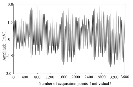
Table 3Influence of different decomposition levels on denoising effect of electromagnetic signal data
Decomposition layer number | SNR | RSTD |
1 | 96.35 | 1.61 |
3 | 95.92 | 1.64 |
5 | 97.99 | 1.54 |
7 | 99.71 | 1.50 |
9 | 97.01 | 1.74 |
11 | 94.39 | 1.91 |
13 | 93.99 | 1.94 |
15 | 93.61 | 1.93 |
Table 4Influence of wavelet basis function selection on denoising effect of electromagnetic signal data
Wavelet function | SNR | RSTD |
Db1 | 96.92 | 1.71 |
Db3 | 95.72 | 1.68 |
Db5 | 96.29 | 1.58 |
Db7 | 97.81 | 1.63 |
Db9 | 98.55 | 1.45 |
sym1 | 95.29 | 1.78 |
sym3 | 95.92 | 1.70 |
sym5 | 95.72 | 1.91 |
sym7 | 95.45 | 2.00 |
sym9 | 95.39 | 1.77 |
From the analysis of Table 3 and Table 4, it can be seen that when the decomposition level is 7, the wavelet transform has the best denoising effect on electromagnetic signal data, and the SNR is 99.71 at the maximum and RSTD is 1.50 at the minimum. When the wavelet function is Db9, the wavelet transform has the best denoising effect on electromagnetic signal data, and the maximum SNR is 98.55 and the minimum RSTD is 1.45. Comprehensive analysis shows that when the decomposition level is 7 and the wavelet function is Db9, the SNR is the largest and RSTD is the smallest, and the wavelet transform has the best denoising effect on electromagnetic signal data.
When wavelet transform is adopted, the decomposition level is set to 7 layers and the wavelet basis function is Db9, and the original electromagnetic signal in Fig. 2 is preprocessed to obtain the denoised electromagnetic signal, as shown in Fig. 3.
Fig. 3Electromagnetic signal after wavelet transform denoising
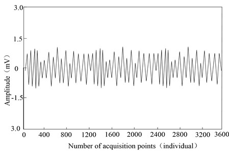
From the analysis of Fig. 3, we can know that the electromagnetic signal denoising can be realized quickly by using wavelet transform. By setting the decomposition level to be 7 and the wavelet basis function to be Db9, the collected original electromagnetic signal is processed according to the decomposition algorithm through wavelet decomposition, and the high-frequency electromagnetic noise signal coefficient is filtered, and the original electromagnetic signal remains valuable after denoising.
Taking the original electromagnetic signal after wavelet transform denoising as the input of convolutional neural network, the electromagnetic signal is modulated and identified by this method, and the accuracy of modulation identification of electromagnetic signal by this method is obtained, as shown in Fig. 4.
Fig. 4The recognition accuracy of electromagnetic signal modulation recognition based on this method
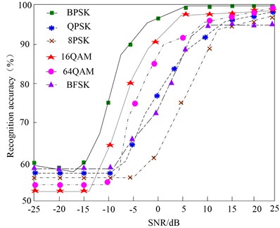
As can be seen from Fig. 4, the modulation recognition rate curve of the electromagnetic signal proposed in this paper is roughly “S”-shaped, that is, the recognition rate is 60 % at low signal-to-noise ratio. With the increase of signal-to-noise ratio, the recognition rate increases rapidly, and it gradually stabilizes and approaches 100 % at high signal-to-noise ratio. Among them, the method in this paper has the best recognition effect on BPSK electromagnetic signal modulation, and the recognition accuracy is obviously improved when SNR = –10 dB, and the recognition accuracy can reach above 98 % when SNR = 5 dB. After SNR = 10 dB, the average accuracy of electromagnetic signal modulation recognition can reach above 97.2 %, which shows that the method in this paper has high accuracy and is suitable for various types of electromagnetic signal modulation recognition.
Using this method to identify the sample data of the test set, the ROC curves of false alarm rate (FPR) and recall rate (TPR) are obtained, as shown in Fig. 5.
Fig. 5ROC Curve of test set
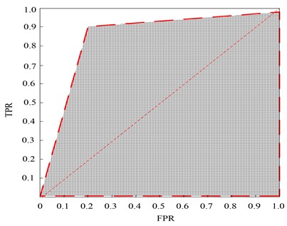
As can be seen from Fig. 5, after classifying the sample data of the test set by the method in this paper, the ROC curve of the test results is highly fitted, and the recall value can reach above 0.97 by solving the ROC curve, while the area under the ROC curve is large. Therefore, in the application process, the Softmax classifier of convolutional neural network proposed in this paper can quickly realize sample sorting and classification recognition, and has strong adaptability.
Fig. 6Changes of loss value with the number of training rounds during CNN training
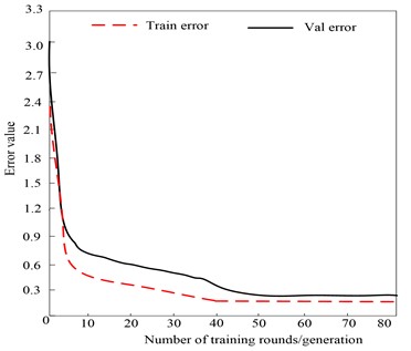
In order to verify the performance of convolutional neural network, in the training process of convolutional neural network, the batch size is 1024, and each training completes an iteration with 86,000 sample points. After each iteration, the data is disrupted, and the next iteration is restarted. After each iteration, the val error will be checked. If the Val error does not change for many times in a row, it indicates that the model parameters are fully trained, then the training process will be terminated and the training results will be output, as shown in Fig. 6.
As can be seen from Fig.6, with the increase of the number of training iterations, both the training set loss value (train error) and the verification set loss value (val error) gradually decrease. When the verification set loss value drops to 0.4-0.5, the verification set loss value hardly changes after the 50th generation, and the network model parameters are fully trained, so the training is over, which shows that the convolutional neural network adopted in this paper has high training efficiency and good robustness.
4. Conclusions
Aiming at the problem that the accuracy of the previous electromagnetic signal modulation identification methods is not high, this paper studies the electromagnetic signal modulation identification method based on wavelet transform convolutional neural network to improve the electromagnetic signal modulation identification ability. The experimental results show that this method can realize the feasibility of electromagnetic signal modulation signal recognition, and the recognition effect is remarkable. Wavelet transform can quickly realize electromagnetic signal denoising, and the collected original electromagnetic signal is processed according to the decomposition algorithm through wavelet decomposition to filter out the high-frequency electromagnetic noise signal coefficients, and the original electromagnetic signal after denoising retains valuable signals. The electromagnetic signal after noise reduction is input into convolutional neural network, and the feature vector of electromagnetic signal modulation signal is effectively extracted through convolutional neural network. In the application process, the Softmax classifier of convolutional neural network can quickly realize sample sorting and classification recognition, and has strong adaptability. As a new intelligent processing method of electromagnetic signals, the method proposed in this paper can also be applied to many potential fields such as radar pulse analysis, radar fingerprint identification, communication signal identification and so on. At the same time, this method is beneficial to improve the cognitive and adaptive ability of complex dynamic electromagnetic environment, as well as the intelligent classification and identification ability of various types of radiation sources.
References
-
Y. Qin and X. Tao, “Research on anti-electromagnetic interference optimization simulation of unmanned aerial vehicle communication channel.,” Nonlinear Optics, Quantum Optics, Vol. 54, 2021.
-
K. F. Ji, J. Gao, Q. J. Wu, and X. Y. Cao, “Research on Vortex electromagnetic wave based on coding metasurface,” in Materials Science Forum, Vol. 1035, No. 12, pp. 724–731, Jun. 2021, https://doi.org/10.4028/www.scientific.net/msf.1035.724
-
T. Li and Y. Xiao, “Domain adaptation-based automatic modulation recognition,” Scientific Programming, Vol. 2021, pp. 1–9, Oct. 2021, https://doi.org/10.1155/2021/4277061
-
C. Liu, L. Chen, and Y. Wu, “Research on signal modulation recognition in wireless communication network by deep learning,” Nonlinear Optics, Quantum Optics, Vol. 55, No. 3-4, pp. 331–341, 2022.
-
C.-H. Shen, “Acoustic emission based grinding wheel wear monitoring: Signal processing and feature extraction,” Applied Acoustics, Vol. 196, p. 108863, Jul. 2022, https://doi.org/10.1016/j.apacoust.2022.108863
-
D. Partington, M. Shanafield, and C. Turnadge, “A comparison of time-frequency signal processing methods for identifying non-perennial streamflow events from streambed surface temperature time series,” Water Resources Research, Vol. 57, No. 9, p. e2020WR028670, Sep. 2021, https://doi.org/10.1029/2020wr028670
-
H. He et al., “Signal Extraction, Transformation, and magnification for ultrasensitive and specific detection of nucleic acids,” Analytical Chemistry, Vol. 93, No. 30, pp. 10611–10618, Aug. 2021, https://doi.org/10.1021/acs.analchem.1c01812
-
S. Kim, H.-Y. Yang, and D. Kim, “Fully complex deep learning classifiers for signal modulation recognition in non-cooperative environment,” IEEE Access, Vol. 10, pp. 20295–20311, Jan. 2022, https://doi.org/10.1109/access.2022.3151980
-
M. Yuan et al., “Rapid classification of steel via a modified support vector machine algorithm based on portable fiber-optic laser-induced breakdown spectroscopy,” Optical Engineering, Vol. 60, No. 12, p. 124114, Dec. 2021, https://doi.org/10.1117/1.oe.60.12.124114
-
A. Dadgarnia and M. T. Sadeghi, “Automatic recognition of pulse repetition interval modulation using temporal convolutional network,” IET Signal Processing, Vol. 15, No. 9, pp. 633–648, Jul. 2021, https://doi.org/10.1049/sil2.12069
-
R. Lei, F. Berto, C. Hu, Z. Lu, and X. Yan, “Early‐warning signal recognition methods in flawed sandstone subjected to uniaxial compression,” Fatigue and Fracture of Engineering Materials and Structures, Vol. 46, No. 3, pp. 955–974, Dec. 2022, https://doi.org/10.1111/ffe.13911
-
A. Ohnishi et al., “Comparison of the pharmacokinetics of E2020, a new compound for Alzheimer’s disease, in healthy young and elderly subjects,” The Journal of Clinical Pharmacology, Vol. 33, No. 11, pp. 1086–1091, Mar. 2013, https://doi.org/10.1002/j.1552-4604.1993.tb01945.x
-
B. G. Palm, F. M. Bayer, and R. J. Cintra, “Signal detection and inference based on the beta binomial autoregressive moving average model,” Digital Signal Processing, Vol. 109, p. 102911, Feb. 2021, https://doi.org/10.1016/j.dsp.2020.102911
-
M. Akilli, N. Yilmaz, and K. Gediz Akdeniz, “Automated system for weak periodic signal detection based on Duffing oscillator,” IET Signal Processing, Vol. 14, No. 10, pp. 710–716, Feb. 2021, https://doi.org/10.1049/iet-spr.2020.0203
-
S. R. Pordanjani, J. Mahseredjian, M. Naïdjate, N. Bracikowski, M. Fratila, and A. Rezaei-Zare, “Electromagnetic modeling of inductors in EMT-type software by three circuit-based methods,” Electric Power Systems Research, Vol. 211, p. 108304, Oct. 2022, https://doi.org/10.1016/j.epsr.2022.108304
-
H. Wei, T. Qi, G. Feng, and H. Jiang, “Comparative research on noise reduction of transient electromagnetic signals based on empirical mode decomposition and variational mode decomposition,” Radio Science, Vol. 56, No. 10, Oct. 2021, https://doi.org/10.1029/2020rs007135
-
Q. Xiao, M. Fan, and X. Zuo, “Speckle phase map denoising based on empirical wavelet transform and cross correlation,” Optical Engineering, Vol. 60, No. 6, p. 064102, Jun. 2021, https://doi.org/10.1117/1.oe.60.6.064102
-
W. K. Ngai, H. Xie, D. Zou, and K.-L. Chou, “Emotion recognition based on convolutional neural networks and heterogeneous bio-signal data sources,” Information Fusion, Vol. 77, pp. 107–117, Jan. 2022, https://doi.org/10.1016/j.inffus.2021.07.007
-
J. Shukla, B. K. Panigrahi, and P. K. Ray, “Power quality disturbances classification based on Gramian angular summation field method and convolutional neural networks,” International Transactions on Electrical Energy Systems, Vol. 31, No. 12, Nov. 2021, https://doi.org/10.1002/2050-7038.13222
-
H. Huang et al., “Clusters induced electron redistribution to tune oxygen reduction activity of transition metal single‐atom for metal-air batteries,” Angewandte Chemie International Edition, Vol. 61, No. 12, Mar. 2022, https://doi.org/10.1002/anie.202116068
Cited by
About this article

The authors have not disclosed any funding.
The datasets generated during and/or analyzed during the current study are available from the corresponding author on reasonable request.
The authors declare that they have no conflict of interest.
