Application of the polynomial dimensional decomposition method in a class of random dynamical systems

Lu, Kuan; Hou, Lei; Chen, Yushu

doi:10.21595/jve.2017.18193

Journal of Vibroengineering

Browse Journal

Submit article

Published: 15 November 2017

Check for updates

Application of the polynomial dimensional decomposition method in a class of random dynamical systems

Kuan Lu¹

Lei Hou²

Yushu Chen³

¹College of Engineering, The University of Iowa, Iowa City, IA 52242, USA

^{1, 2, 3}School of Astronautics, Harbin Institute of Technology, Harbin 150001, P. R. China

²School of Energy Science and Engineering, Harbin Institute of Technology, Harbin 150001, P. R. China

Corresponding Author:

Kuan Lu

Cite the article Download PDF

Downloads 1576

WoS Core Citations 4

CrossRef Citations 4

Abstract

The polynomial dimensional decomposition (PDD) method is applied to study the amplitude-frequency response behaviors of dynamical system model in this paper. The first two order moments of the steady-state response of a dynamical random system are determined via PDD and Monte Carlo simulation (MCS) method that provides the reference solution. The amplitude-frequency behaviors of the approximately exact solution obtained by MCS method can be retained by PDD method except the interval close to the resonant frequency, where the perturbations may occur. First, the results are shown on the two degrees of freedom (DOFs) spring system with uncertainties; the dynamic behaviors of the uncertainties for mass, damping, stiffness and hybrid cases are respectively studied. The effects of PDD order to amplitude-frequency behaviors are also discussed. Second, a simple rotor system model with four random variables is studied to further verify the accuracy of the PDD method. The results obtained in this paper show that the PDD method is accurate and efficient in the dynamical model, providing the theoretical guidance to complexly nonlinear rotor dynamics models.

1. Introduction

The dynamical analysis of multiple DOF (MDOF) nonlinear system has become one central issue of concerns in dynamics, attracting the significant attention of researchers in many areas. The calculating quantity of the MDOF system is extremely huge and the qualitative analysis can’t provide comprehensive guidance, so the reduced models obtained by order reduction methods are necessary. Then the numerical simulation and theoretical analysis on the reduced model will be less expensive and more clearly. A series of efficient order reduction methods can be applied in actual high-dimensional system. For example, center manifold method [1, 2], inertial manifold method [3], POD method [4-8], Galerkin method [9, 10], Lyapunov-Schmidt method [11, 12], and other order reduction methods [13], which were summarized by Rega [14] and Steindle [15] in dynamic research. These methods are usually valid in deterministic systems and will be out of action in uncertain systems.

The physical parameters of engineering systems may change in an uncertain way because of considering design uncertainty and the variance of system response is also uncertain. The goal is to allow an estimate of dynamic responses generated by these considerations on physical parameters. There are a variety of methods in a view of uncertainties for this type of issues: such as the perturbation method [16, 17], Neumann method [18, 19], MCS method [20-22], polynomial chaos expansion (PCE) method [23-25], and PDD method [26-28]. The perturbation method is based on the expansion of random quantities into Taylor series [29], and the Neumann method is on the basis of Neumann series [30, 31], they can both solve the small random fluctuations problems but do not fit for the case close to the resonant frequency. Monte Carlo simulation is an exact method to obtain approximately accurate solutions of the uncertain system. But the MCS’s calculated amount is very large in case of corresponding large samples [32]. The PCE and PDD are both efficient uncertain quantification methods, which are widely used in the high-dimensional complex systems [33, 34].

The PCE approximation commits a larger error than the PDD approximation for identical expansion orders when the cooperative efforts of input variables on an eigenvalue attenuate rapidly or vanish altogether [35]. The accuracy and efficiency of PDD is verified by some numerical results in comparison to PCE [36, 37]. The PDD method is a good way to study uncertain problems, so the PDD method is chosen to solve dynamical systems with uncertainties in this paper.

The motivation of this paper is to generalize the PDD method to dynamical system models with uncertainties. The random dynamic system response and brief introduction to PDD method are provided in Section 2. A spring model of two DOF is established in Section 3. In Section 4, the amplitude frequency behaviors of the spring system model with uncertainties of design parameters are discussed to verify the efficiency of the PDD method via comparing with the Monte Carlo simulation method, and the influence of the PDD’s approximation order is highlighted. The PDD method is generalized to linear system model in Section 5. Finally, the conclusions and outlooks are drawn in Section 6.

2. Response of random dynamic system with harmonic excitation

The dynamical system with uncertainties will be introduced in this section, and then the PDD method will be used to solve the dynamical equation.

2.1. Design uncertainties in a dynamical system

In general, the $n \times n$ mass matrix $M$ , damping matrix $C$ , and stiffness matrix $K$ can describe the dynamical system, where $n$ is the DOF number. The external excitation force of the system can be denoted as $F (t)$ , and $y (t)$ is DOF vector.

We consider that the mass, damping and stiffness matrices are uncertain, which can be expressed as:

1

M = \underline{M} (1 + c o v_{M} δ_{M}),

2

C = \underline{C} (1 + c o v_{C} δ_{C}),

3

K = \underline{K} (1 + c o v_{K} δ_{K}) .

The parameters in Eqs. (1-3) are shown as follows: $c o v_{M}$ – cov of mass, $δ_{M}$ – standard normal deviate of mass, $c o v_{C}$ – cov of damping, $δ_{C}$ – standard normal deviate of damping, $c o v_{K}$ – cov of stiffness, $δ_{K}$ – standard normal deviate of stiffness.

The system is deterministic when the coefficient of variance (cov) is zero. We choose simple uncertainty to show the motivation of this paper. On the basis of the PDD method, the dynamic behaviors around the resonant frequencies will be highlighted. It should be specified that the PDD method is generalized to solve the dynamical problems for the first time. On account of actually physical significance, Gaussian distribution may lead to negative values of the design parameters, so the control parameters are considered to be very small, design parameters won’t be negative. The PDD method can also be applied in other distribution (Uniform, Beta distribution, etc.), we don’t discuss in details here.

In general, dynamical equation can be expressed as:

4

M \ddot{y} (t) + C \dot{y} (t) + K y (t) = F (t) .

We consider the external excitation to be harmonic $F (t) = F_{0} e^{i ω t}$ , the steady state response of system is assumed to be $y (t) = Y e^{i ω t}$ , $i = \sqrt{- 1}$ , and $Y$ is the solution of Eq. (5):

5

(- ω^{2} M + i ω C + K) Y = F_{0} .

The matrixes $M$ , $C$ , $K$ and $Y$ are random, which can be described by the moments of the system. The mean and standard deviation (SD) of the system response are calculated. The calculating formulas of the first two order moments are provided in Ref. [38]. The amplitude of the amplitude-frequency response function can be denoted as $|Y_{1} + i Y_{2}|$ , where $Y_{1}$ and $Y_{2}$ are the real and imaginary part of $Y$ respectively.

Actually, both MCS and PDD methods can be applied to derive these moments. The results obtained by MCS method can provide reference solutions and the PDD method will be used to compare with the MCS method in this paper.

The PDD method is an efficient uncertain quantification method for order reduction in the stochastic systems [26], an $S$ -variate approximation PD of the response $y (x)$ , described by [39]:

6

\begin{array}{l} {\tilde{y}}_{S} (x) = y_{0} + \sum_{i = 1}^{N} y_{i} (x_{i}) + \sum_{i_{1}, i_{2} = 1; i_{1} < i_{2}}^{N} y_{i_{1} i_{2}} (x_{i_{1}}, x_{i_{2}}) + \sum_{i_{1}, i_{2}, i_{3} = 1; i_{1} < i_{2} < i_{3}}^{N} y_{i_{1} i_{2} i_{3}} (x_{i_{1}}, x_{i_{2}}, x_{i_{3}}) \\ + \dots + \sum_{i_{1}, \dots, i_{S} = 1; i_{1} < \dots i_{S}}^{N} y_{i_{1} \dots i_{S}} (x_{i_{1}}, \dots, x_{i_{S}}) . \end{array}

Eq. (6) can be regarded as a finite hierarchical expansion of an output function in terms of the input variables with the increasing dimensions, and $y_{0}$ is a constant, $y_{i} (x_{i})$ is a univariate component function that represents individual contribution to $y (x)$ by input variable $x_{i}$ acting alone. In a similar way, $y_{i_{1} i_{2}} (x_{i_{1}}, x_{i_{2}})$ is a bivariate component function, $y_{i_{1} i_{2} i_{3}} (x_{i_{1}}, x_{i_{2}}, x_{i_{3}})$ is trivariate and $y_{i_{1} \dots i_{S}} (x_{i_{1}}, \dots, x_{i_{S}})$ is an $S$ -variate component function. The response converges to the exact function $y (x)$ , when $S \to N$ .

The approximate expressions of the first three variate component functions are given, which are described by:

7

y_{i} (x_{i}) ≅ \sum_{j = 1}^{m} α_{i j} ψ_{i j} (x_{i}),

8

y_{i_{1} i_{2}} (x_{i_{1}}, x_{i_{2}}) ≅ \sum_{j_{2} = 1}^{m} \sum_{j_{1} = 1}^{m} β_{i_{1} i_{2} j_{1} j_{2}} ψ_{i_{1} j_{1}} (x_{i_{1}}) ψ_{i_{2} j_{2}} (x_{i_{2}}),

9

y_{i_{1} i_{2} i_{3}} (x_{i_{1}}, x_{i_{2}}, x_{i_{3}}) ≅ \sum_{j_{3} = 1}^{m} \sum_{j_{2} = 1}^{m} \sum_{j_{1} = 1}^{m} γ_{i_{1} i_{2} i_{3} j_{1} j_{2} j_{3}} ψ_{i_{1} j_{1}} (x_{i_{1}}) ψ_{i_{2} j_{2}} (x_{i_{2}}) ψ_{i_{3} j_{3}} (x_{i_{3}}) .

The corresponding coefficients are the parameters $α_{i j}$ , $β_{i_{1} i_{2} j_{1} j_{2}}$ , $γ_{i_{1} i_{2} i_{3} j_{1} j_{2} j_{3}}$ , you can see details in Ref. [26].

2.2. Dynamical equation on the basis of PDD

As above, $y (t)$ is the random DOF vector, which is a solution of the Eq. (4), and $M$ , $C$ , $K$ are expressed as Eqs. (1) to (3). An $S$ -variate approximation of the PDD of response $y (X)$ can be described by:

10

\begin{array}{l} {\tilde{y}}_{S} (X) ≅ y_{0} + \sum_{i = 1}^{N} \sum_{j = 1}^{m} α_{i j} ψ_{i j} (X_{i}) + \sum_{i_{1}, i_{2} = 1; i_{1} < i_{2}}^{N} \sum_{j_{2} = 1}^{m} \sum_{j_{1} = 1}^{m} β_{i_{1} i_{2} j_{1} j_{2}} ψ_{i_{1} j_{1}} (X_{i_{1}}) ψ_{i_{2} j_{2}} (X_{i_{2}}) \\ + \sum_{i_{1}, i_{2}, i_{3} = 1; i_{1} < i_{2} < i_{3}}^{N} \sum_{j_{3} = 1}^{m} \sum_{j_{2} = 1}^{m} \sum_{j_{1} = 1}^{m} γ_{i_{1} i_{2} i_{3} j_{1} j_{2} j_{3}} ψ_{i_{1} j_{1}} (X_{i_{1}}) ψ_{i_{2} j_{2}} (X_{i_{2}}) ψ_{i_{3} j_{3}} (X_{i_{3}}) \\ + \dots + \sum_{i_{1}, \dots, i_{S} = 1; i_{1} < \dots < i_{S}}^{N} \sum_{j_{S} = 1}^{m} \dots \sum_{j_{1} = 1}^{m} C_{i_{1}, \dots, i_{S} j_{1}, \dots, j_{S}} \prod_{k = 1}^{S} ψ_{i_{k} j_{k}} (X_{i_{k}}) . \end{array}

In the case of $S = N$ , Eq. (10) will converge to $y (X)$ in the mean square sense as $m \to \infty$ . We apply the dimension reduction integration method [40] to calculate $y_{0}$ and $C_{i_{1}, \dots, i_{S} j_{1}, \dots, j_{S}}$ . We use only the univariate method to study the simple models in this paper. So, the corresponding coefficients are:

11

y_{0} = \int_{I R^{N}} y (\underline{x}) ϕ (\underline{x}) d \underline{x} ≅ \sum_{i = 1}^{N} \int_{- \infty}^{+ \infty} y (0, \dots, 0, x_{i}, 0, \dots, 0) ϕ (x_{i}) d x_{i} - (N - 1) y (\underline{0}),

12

α_{i j} = \int_{I R^{N}} y (\underline{x}) φ_{i j} (x_{i}) ϕ (\underline{x}) d \underline{x} ≅ \int_{- \infty}^{+ \infty} y (0, \dots, 0, x_{i}, 0, \dots, 0) φ_{i j} (x_{i}) d x_{i} .

The dynamical systems in this manuscript are linear and contain at most four random variables, so the univariate method is enough.

The calculating formulas of response moments of the PDD method are written as Eqs. (13) and (14). In this paper, we only use the first and second order moment, so the formulas of first two order moments are listed as follows:

13

E [{\tilde{y}}_{S} (X)] = y_{0},

14

E {[{\tilde{y}}_{S} (X) - y_{0}]}^{2} = \sum_{s = 1}^{S} (\sum_{i_{1} = 1}^{N - s + 1} \dots \sum_{i_{s} = i_{s - 1} + 1}^{N} \sum_{j_{1} = 1}^{m} \dots \sum_{j_{s} = 1}^{m} C_{i_{1}, \dots, i_{s} j_{1}, \dots, j_{s}}^{2}) .

As mentioned above, the PDD components can satisfy the form of Eq. (15):

15

\bar{\bar{M}} \ddot{\bar{x}} (t) + \bar{\bar{C}} \dot{\bar{x}} (t) + \bar{\bar{K}} \ddot{\bar{x}} (t) = \bar{\bar{F}} (t) .

So, the dynamical system with uncertainty can be regarded as the deterministic one. Then we can apply PDD method to study the stochastic moments of the amplitude-frequency response of the dynamical system.

Remark 1. The common design uncertainties of general dynamic system are listed, such as the mass, damping, stiffness. We use the simple uncertainty (normal distribution) to highlight the specially dynamical characteristics close to resonant frequencies obtained by the PDD method. In the previous studies of other researchers, they all use the PCE method, but the PCE method has a larger error than the PDD method. This paper generalizes the PDD method to solve the dynamical problems.

3. Two-DOF spring system model

A two-DOF spring system model will be established which is shown in Fig. 1, the PDD and MCS methods will be applied to calculate the first two order moments of steady state response. The total cost of MCS method is more expensive than the PDD method, the advances of the PDD method will be discussed briefly in Section 4.

Fig. 1Two-DOF spring model

The dynamical equation of the spring system model is similar as Eq. (4), the parameters are expressed as follows:

16

M = (\begin{array}{l} m_{1} \\ m_{2} \end{array}), C = (\begin{matrix} c_{1} + c_{2} & - c_{2} \\ - c_{2} & c_{2} + c_{3} \end{matrix}), K = (\begin{matrix} k_{1} + k_{2} & - k_{2} \\ - k_{2} & k_{2} + k_{3} \end{matrix}), F (t) = (\begin{array}{l} F_{1} \\ F_{2} \end{array}) .

The design parameters are all assumed to be uncertain and they are considered to be equal to each other. The stiffness, damping and the mass are denoted as $k$ , $c$ and $m$ respectively. See the values in details in Table 1.

The formulas of uncertain parameters are written as Eqs. (15)-(17):

17

m = \bar{m} (1 + c o v_{m} δ_{m}),

18

c = \bar{c} (1 + c o v_{c} δ_{c}),

19

k = \bar{k} (1 + c o v_{k} δ_{k}) .

The parameters $c o v_{m}$ , $c o v_{c}$ , $c o v_{k}$ are the cov parameters and $\bar{m}$ , $\bar{c}$ , $\bar{k}$ are the mean values.

Remark 2. The 2-DOF spring model is selected to study dynamic behaviors of the stochastic system. We consider that the response and external excitation are harmonic, see details in Section 2. So, we can study the analytical behaviors to highlight the efficiency of the PDD method. We will also choose a linear rotor system model to further verify the accuracy of the PDD method.

Table 1Corresponding values

$m$ (kg)	$c$ (Nm^-1s^-1)	$k$ (Nm^-1)	$c o v_{m}$	$c o v_{c}$	$c o v_{k}$	$F_{1}$ (N)	$F_{2}$ (N)
1	1	15000	3 %	4 %	5 %	1	0

4. Dynamical characteristics of the spring system

The sole design (stiffness, damping or stiffness) uncertainty is studied first in this section. Then the amplitude-frequency response characteristics of the hybrid uncertainty cases are discussed. The DOF vector is calculated for 1001values of $ω / (2 π)$ in the domain from 15 Hz to 40 Hz.

The MCS results are obtained with 10000 samples of the random variables $δ_{m}$ , $δ_{c}$ , $δ_{k}$ . The first two order moments are plotted in Fig. 2 to Fig. 8. The PDD order is calculated in the cases of 2 and 9 to verify the effects of PDD order.

We discuss the advances of the PDD method briefly here. We need to call the response of the system 10000 times via using the MCS method. In comparison to MCS method, the times (PDD method) you call the response are $\sum_{k = 0}^{k = R} (\begin{matrix} N \\ R - k \end{matrix}) {(n - 1)}^{R - k}$ , etc., the univariate PDD is $(n - 1) N + 1$ , where $N$ is the number of uncertain quantities and $n$ is the number of integration points. The MCS method is more expensive than the univariate PDD, so we choose PDD method to study the response of the stochastic dynamics systems [26].

4.1. Stiffness uncertainty

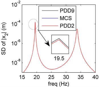
In case of PDD order 2 and 9, the first two order moments of the system are plotted in Fig. 2, the mean reserves the amplitude-frequency trend of the MCS result, and the SD meets well with the MCS result. Both mean and SD calculated by PDD have oscillations close to the resonance. As the PDD order increases, the curves oscillate more and the vibration amplitude decreases.

Fig. 2Amplitude frequency curves of PDD2 (red line), PDD9 (black line) and MCS (blue line)

a) Mean of PDD

b) SD of PDD

4.2. Damping uncertainty

In Fig. 3, the spring system model with damping uncertainty is discussed. The PDD results of mean are in good agreement with the MCS results, and the oscillations disappear. Compared with the mean results, the SD values agree well with the MCS results, the higher PDD order has little effect to the dynamical characteristics.

As usual, variation of damping has little effect to the position of resonant frequency of dynamical system, so the resonant frequencies of mean and SD values keep almost the same. Amplitude usually varies as the damping in dynamical system, and the results in Fig. 3 verify this case. At present, the cause leads to the disappearing of PDD oscillations is not clear, we can regard this as a research topic in the future.

Fig. 3Amplitude frequency curves of PDD2 (red line), PDD9 (black line) and MCS (blue line)

a) Mean of PDD

b) SD of PDD

4.3. Mass uncertainty

Similar as the stiffness and damping uncertainties, the amplitude-frequency curves of the mass uncertainty case are plotted in Fig. 4. The SD values obtained by the PDD method are in great agreement with the MCS results. In the case of higher PDD order (the order is 9), the PDD results can approximate to the exact results better than the order 2 case.

Fig. 4Amplitude frequency curves of PDD2 (red line), PDD9 (black line) and MCS (blue line)

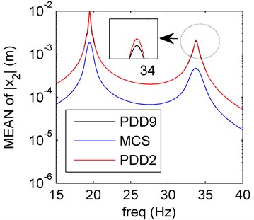
a) Mean of PDD

b) SD of PDD

Remark 3. The dynamic behaviors of spring system model with three cases of uncertain design parameters are studied. The first two order moments of the system are calculated by the PDD method to compare with the MCS results so as to verify PDD method’s accuracy. The oscillations of PDD results occur near the frequency of resonance and increase as the PDD order increase. In the case of higher PDD order, the amplitude decreases, the PDD method reserves the amplitude-frequency characteristics better. The damping uncertainty of the PDD results has minimum effect compared with the mass and stiffness uncertainties, there is almost no oscillation, and the SD curves have perfect agreement with the MCS results.

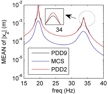
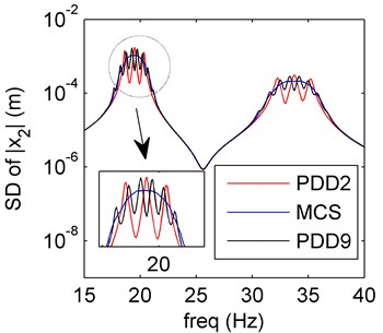
4.4. Hybrid uncertainty

The hybrid uncertainty case of spring system model will be discussed in this section. See the uncertain parameter values and the order number in Table 2.

Table 2Corresponding uncertain parameters and the order

Case	$δ_{k}$	$δ_{c}$	$δ_{m}$	Order	Order
1	0.05	0.04		2	9
2	0.05		0.03	2	9
3		0.04	0.03	2	9
4	0.05	0.04	0.03	2	9

4.4.1. Case 1

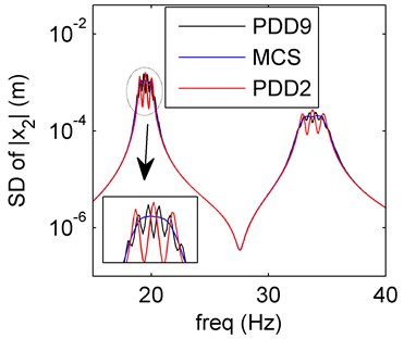
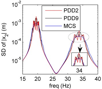
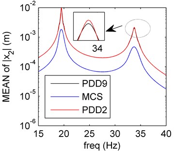
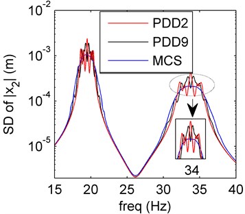
Similar as the previous discussion, the SD curves based on the PDD method have good agreement with the MCS results except for the frequencies around the resonant frequency (see Fig. 5). The amplitude values decrease as PDD order increases, the approximation of the PDD results to the MCS results are better. The mean and SD oscillate more than the sole damping uncertainty (Section 4.2).

4.4.2. Case 2

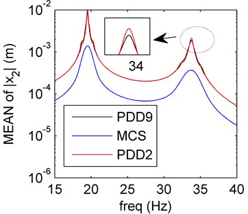
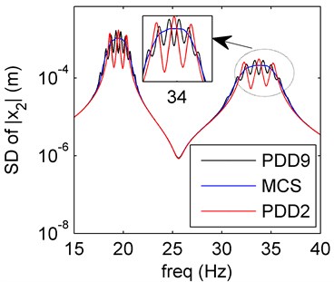
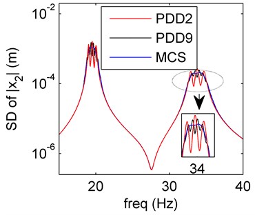
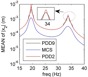
In Fig. 6(a), the amplitude frequency response behaviors of PDD results of the mean reserve the dynamical trend of the MCS results, and the PDD order 9 approximates better than the order 2. The PDD results of the SD can also reserve amplitude-frequency characteristics of the MCS results better in Fig. 6(b), but the results oscillate more than the sole mass or stiffness uncertainty, the amplitude-frequency characteristics are more complex than the cases we previously discussed. So, we can draw a conclusion that the hybrid uncertainties (both mass and stiffness) are more sensitive than the sole uncertainty (Sections 1 and 3). On the basis of such complex uncertainties, the PDD results can also have perfect agreement with the MCS results and the results are better when the PDD order increases.

Fig. 5Amplitude frequency curves of PDD2 (red line), PDD9 (black line) and MCS (blue line)

a) Mean of PDD

b) SD of PDD

Fig. 6Amplitude frequency curves of PDD2 (red line), PDD9 (black line) and MCS (blue line)

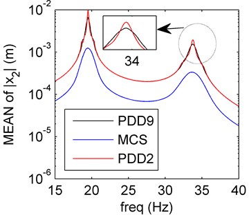
a) Mean of PDD

b) SD of PDD

4.4.3. Case 3

Both damping and mass uncertainties are discussed here. We want to compare case 3 with the sole damping uncertainty (Section 4.2). In Fig. 7, the mean and SD of PDD results oscillate more than those in Fig. 3. To compare the case 3 with case 1 and 2, both the stiffness (compare case 2 with 3) and mass (compare case 1 with 2) uncertainties affect more than the damping uncertainty.

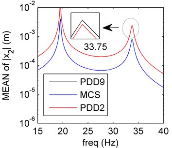
4.4.4. Case 4

In Fig. 8, it is clear that the first two order moments obtained by PDD method are almost the same as those of case 2. The PDD results can meet the exact solutions very well. The results based on three uncertain variables all reveal that the damping uncertainty have little effect to the system.

Remark 4. The amplitude frequency response behaviors of the spring system model with hybrid uncertainties are studied in four cases (1-4). In case 1 and 3, the stiffness and mass uncertainties have larger effect compared with the solely damping uncertainty (Section 4.2), the oscillation occur around the resonance. The case 4 contains three uncertain variables (mass, damping and stiffness), which oscillates more than case 1 and 3, the damping uncertainty has little effect to the system. Meanwhile, the PDD results can agree better with the MCS ones as the PDD order increases. The mass and stiffness uncertainties are more sensitive than the damping uncertainty.

Fig. 7Amplitude frequency curves of PDD2 (red line), PDD9 (black line) and MCS (blue line)

a) Mean of PDD

b) SD of PDD

Fig. 8Amplitude frequency curves of PDD2 (red line), PDD9 (black line) and MCS (blue line)

a) Mean of PDD

b) SD of PDD

5. Dynamic behaviors of the linear rotor system

The PDD method will be used to study amplitude frequency behaviors of the linear rotor system with uncertain quantities preliminarily in this section. We will only discuss the amplitude frequency response behaviors of the system in the case of PDD order 2, and other complex cases will be studied in details in the authors’ future work.

5.1. HB method in rotor system

The rotor system model in this paper is similar as one of the authors’ previous work, see details in Ref. [8]. The nonlinear stiffness term is neglected, so the model we discussed as follows is a linear case, the dynamical equation can be expressed as Eq. (1) in Ref. [8], and we don’t provide the equation here. We will use the HB-1 method to solve the response of the rotor system when the Fourier series order is 1. The response is considered as follows:

20

\tilde{\underline{y}} = {\underline{A}}_{0} + {\underline{A}}_{1} c o s ω t + {\underline{B}}_{1} s i n ω t,

21

\underline{F} (t) = {\underline{F}}_{0} + {\underline{F}}_{1} c o s ω t + {\underline{F}}_{2} s i n ω t .

Hence, we can get the equations as follows:

22

\dot{\tilde{\underline{y}}} = - {\underline{A}}_{1} ω s i n ω t + {\underline{B}}_{1} ω c o s ω t,

23

\ddot{\tilde{\underline{y}}} = - {\underline{A}}_{1} ω^{2} c o s ω t - {\underline{B}}_{1} ω^{2} s i n ω t,

where:

{\underline{F}}_{0} = {(\begin{array}{l} 0 & - m_{1} g & 0 & - m_{2} g & 0 & - m_{3} g \end{array})}^{T}, {\underline{F}}_{1} = {(\begin{array}{l} 0 & 0 & m_{2} e ω^{2} & 0 & 0 & 0 \end{array})}^{T},

{\underline{F}}_{2} = {(\begin{array}{l} 0 & 0 & 0 & m_{2} e ω^{2} & 0 & 0 \end{array})}^{T} .

Substitute Eqs. (20)-(23) into Eq. (4), we can get:

24

\underline{K} {\underline{A}}_{0} = {\underline{F}}_{0},

25

\underline{K} {\underline{A}}_{1} + \underline{C} {\underline{B}}_{1} ω - \underline{M} {\underline{A}}_{1} ω^{2} = {\underline{F}}_{1},

26

\underline{K} {\underline{B}}_{1}_{1} - \underline{C} {\underline{A}}_{1} ω - \underline{M} {\underline{B}}_{1}_{1} ω^{2} = {\underline{F}}_{2} .

We neglect the static part, and we can obtain the Eq. (27):

27

{(\begin{matrix} \underline{K} - \underline{M} ω^{2} & \underline{C} ω \\ - \underline{C} ω & \underline{K} - \underline{M} ω^{2} \end{matrix})}_{12 \times 12} {(\begin{array}{l} {\underline{A}}_{1} \\ {\underline{B}}_{1} \end{array})}_{12 \times 1} = {(\begin{array}{l} {\underline{F}}_{1} \\ {\underline{F}}_{2} \end{array})}_{12 \times 1} .

In Eq. (27):

{\underline{A}}_{1} = {(\begin{array}{l} A_{11} & A_{12} & A_{13} & A_{14} & A_{15} & A_{16} \end{array})}^{T}, {\underline{B}}_{1}_{1} = {(\begin{array}{l} B_{11} & B_{12} & B_{13} & B_{14} & B_{15} & B_{16} \end{array})}^{T} .

The response can be obtained via calculating Eq. (27), then we can get the amplitude in Eq. (28):

28

{\tilde{\underline{y}}}_{i} = \sqrt{{A_{1 i}}^{2} + {B_{1 i}}^{2}}, (i = 1,2, \dots, 6) .

5.2. Four random variables case

In this section, we discuss the four random variables case. The uncertain values and the parameters are shown in the Table 3.

Table 3The parameter values of the rotor system

$m_{1}$	$m_{2}$	$m_{3}$	$c_{1}$	$c_{2}$	$c_{3}$	$k_{1}$	$k_{2}$	$e$ (mm)	$ξ_{\underline{M}}$	$ξ_{\underline{C}}$	$ξ_{\underline{K}}$	$ξ_{e}$
4	30	4	1050	2100	1050	2×10⁶	2×10⁶	0.01	10 %	10 %	10 %	10 %

The mass matrix $\underline{M}$ , stiffness matrix $\underline{K}$ , damping matrix $\underline{C}$ each contains one random variable respectively, and the eccentricity $e$ contains one random variable. So, there are four random variables in this six-DOF rotor system, we don’t write in details in this paper.

The PDD is calculated in the case of polynomial order 2, and the results are reflected in Fig. 9. The mean and SD values for PDD agree well with results of MCS method. It seems that the PDD results will approximate to the approximately exact results better as the polynomial order increases. The results in the rotor system with four random variables further verify the accuracy of the PDD method.

Fig. 9Amplitude frequency curves of PDD (red line) and MCS (blue line)

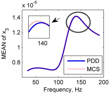
a) Mean of PDD

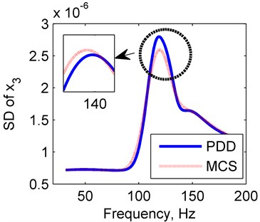
b) SD of PDD

6. Conclusions

The PDD method has been used to study the amplitude frequency response behaviors of the dynamical system with uncertainties for the first time. A two DOF spring system has been established by the Newton’s second law, and the amplitude-frequency characteristics of different system design parameters with uncertainties have been respectively discussed. The results show that both the stiffness and mass uncertainties are more sensitive than the damping uncertainty. The accuracy and efficiency of the PDD method has been verified in comparison to MCS method. The effects of PDD order to order reduction accuracy have also been discussed. A linear rotor system model has been applied to further verify the efficiency of the PDD method. Further work on this subject will be carried out by the authors in three aspects: the first is to eliminate the perturbations around the resonant frequency and the cause of damping leads to the disappearing of PDD oscillations; the second is to generalize the PDD method to the nonlinear rotor systems; the third is to combine the POD and PDD method to reduce the dimension and order of the complex nonlinear rotor systems.

References

Alho A., Uggla C. Global dynamics and inflationary center manifold and slow-roll approximants. Journal of Mathematical Physics, Vol. 56, 2015, p. 012502.

Publisher
Valls C. Center problem in the center manifold for quadratic and cubic differential systems in R³. Applied Mathematics and Computation, Vol. 251, 2015, p. 180-191.

Search CrossRef
Chung Y. M., Steyer A., et al. Global error analysis and inertial manifold reduction. Journal of Computational and Applied Mathematics, Vol. 307, 2016, p. 204-215.

Publisher
Peng L. Q., Mohseni K. Nonlinear model reduction via a locally weighted POD method. International Journal for Numerical Methods in Engineering, Vol. 106, 2016, p. 372-396.

Publisher
Lu K., Yu H., Chen Y. S., Cao Q. J., Hou L. A modified nonlinear POD method for order reduction based on transient time series. Nonlinear Dynamics, Vol. 79, 2015, p. 1195-1206.

Publisher
Lu K., Jin Y. L., Chen Y. S., Cao Q. J., Zhang Z. Y. Stability analysis of reduced rotor pedestal looseness fault model. Nonlinear Dynamics, Vol. 82, 2015, p. 1611-1622.

Publisher
Lu K., Chen Y. S., Jin Y. L., Hou L. Application of the transient proper orthogonal decomposition method for order reduction of rotor systems with faults. Nonlinear Dynamics, Vol. 86, 2016, p. 1913-1926.

Publisher
Lu K., Chen Y. S., Cao Q. J., Hou L., Jin Y. L. Bifurcation analysis of reduced rotor model based on nonlinear transient POD method. International Journal of Non-Linear Mechanics, Vol. 89, 2017, p. 83-92.

Publisher
Frank, Reuter, et al. FESTUNG: A Matlab/GNU Octave toolbox for the discontinuous Galerkin method. Part I: Diffusion operator. Computers and Mathematics with Applications, Vol. 70, 2015, p. 11-46.

Search CrossRef
Zhu J., Zhong X. H., et al. Runge-Kutta discontinuous Galerkin method with a simple and compact Hermite WENO limiter. Communications in Computational Physics, Vol. 19, 2016, p. 944-969.

Publisher
Li C. P., Ma L. Lyapunov-Schmidt reduction for fractional differential systems. Journal of Computational and Nonlinear Dynamics, Vol. 11, 2016, p. 051022.

Publisher
Guo S. J., Yan S. L. Hopf bifurcation in a diffusive Lotka-Volterra type system with nonlocal delay effect. Journal of Differential Equations, Vol. 260, 2016, p. 781-817.

Publisher
Hamilton N., Tutkun M., Cal R. B. Low-order representations of the canonical wind turbine array boundary layer via double proper orthogonal decomposition. Physics of Fluids, Vol. 28, 2016, p. 025103.

Publisher
Rega G., Troger H. Dimension reduction of dynamical systems: methods, models, applications. Nonlinear Dynamics, Vol. 41, 2005, p. 1-15.

Publisher
Steindl A., Troger H. Methods for dimension reduction and their application in nonlinear dynamics. International Journal of Solids and Structures, Vol. 38, 2001, p. 2131-2147.

Publisher
Guo M. W., Zhong H. Z., You K. A second-order perturbation method for fuzzy eigenvalue problems. Engineering Computations, Vol. 33, 2016, p. 306-327.

Publisher
Esparza D. M., Kosovic B., et al. A stochastic perturbation method to generate inflow turbulence in large-eddy simulation models: application to neutrally stratified atmospheric boundary layers. Physics of Fluids, Vol. 27, 2015, p. 035102.

Publisher
Yuan J., et al. A novel hybrid Neumann expansion method for stochastic analysis of mistuned bladed discs. Mechanical Systems and Signal Processing, Vols. 72-73, 2016, p. 241-253.

Publisher
Wang X. Y., Cen S., Li C. F. Generalized Neumann expansion and its application in stochastic finite element methods. Mathematical Problems in Engineering, 2013, p. 325025.

Publisher
Li M. Q., Yang F. A metamodel-based Monte Carlo simulation approach for responsive production planning of manufacturing systems. Journal of Manufacturing System, Vol. 38, 2016, p. 114-133.

Publisher
Wang P., Barajas-Solano D. A., et al. Probabilistic density function method for stochastic ODEs of power systems with uncertain power input. SIAM/ASA Journal on Uncertainty Quantification, Vol. 3, 2015, p. 873-896.

Publisher
Bao N., Wang C. J. A Monte Carlo simulation based inverse propagation method for stochastic model updating. Mechanical Systems and Signal Processing, Vols. 60-61, 2015, p. 928-944.

Publisher
Xie Q. M., Wang J. H., et al. An optimization method for the distance between exits of buildings considering uncertainties based on arbitrary polynomial chaos expansion. Reliability Engineering and System Safety, Vol. 154, 2016, p. 188-196.

Publisher
Jacquelin E., Friswell M. I., et al. Polynomial chaos expansion with random and fuzzy variables. Mechanical Systems and Signal Processing, Vol. 75, 2016, p. 41-56.

Publisher
Peng J., Hampton J., Doostan A. On polynomial chaos expansion via gradient-enhanced ℓ1-minimization. Journal of Computational Physics, Vol. 310, 2016, p. 440-458.

Publisher
Rahman S. A polynomial dimensional decomposition for stochastic computing. International Journal for Numerical Methods in Engineering, Vol. 76, 2008, p. 2091-2116.

Publisher
Sobol I. M. Theorems and examples on high dimensional model representations. Reliability Engineering and System Safety, Vol. 79, 2003, p. 187-193.

Publisher
Hoeffding W. A class of statistics with asymptotically normal distribution. The Annals of Mathematical Statistics, Vol. 19, 293, p. 325-1948.

Publisher
Nayfeh A. Perturbation Methods. John Wiley and Sons, London, 1973.

Search CrossRef
Benaroya H., Rehak M. Finite elements methods in probabilistic structural analysis: a selective review. Applied Mechanics Reviews, Vol. 41, 1988, p. 201-213.

Publisher
Yamazaki F., Shinozuka M., Dasgupta G. Neumann expansion for stochastic finite element analysis. Journal of Engineering Mechanics, Vol. 114, 1988, p. 1335-1354.

Publisher
Didier J., Sinou J. J., Faverjon B. Study of the non-linear dynamic response of a rotor system with faults and uncertainties. Journal of Sound and Vibration, Vol. 31, 2012, p. 671-703.

Publisher
Wiener N. The homogeneous chaos. American Journal of Mathematics, Vol. 60, 897, p. 936-1938.

Publisher
Rahman S. The f-sensitivity index. SIAM/ASA Journal on Uncertainty Quantification, Vol. 4, 2016, p. 130-162.

Publisher
Rahman S., Yadav V. Orthogonal polynomial expansions for solving random eigenvalue problems. International Journal for Uncertainty Quantification, Vol. 1, 2011, p. 163-187.

Publisher
Yadav V. Novel Computational Methods for Solving High-Dimensional Random Eigenvalue Problems. Ph.D. Thesis, University of Iowa, 2013.

Search CrossRef
Yadav V., Rahman S. Adaptive-sparse polynomial dimensional decomposition methods for high-dimensional stochastic computing. Computer Methods in Applied Mechanics Engineering, Vol. 274, 2014, p. 56-83.

Publisher
Rahman S. Statistical moments of polynomial dimensional decomposition. Journal of Engineering Mechanics, Vol. 136, 2010, p. 923-927.

Publisher
Xu H. Q., Rahman S. Decomposition methods for structural reliability analysis. Probabilistic Engineering Mechanics, Vol. 20, 2005, p. 239-250.

Publisher
Xu H. Q., Rahman S. A generalized dimension-reduction method for multi-dimensional integration in stochastic mechanics. International Journal for Numerical Methods in Engineering, Vol. 61, 2004, p. 1992-2019.

Publisher

Cited by

Random vibration analysis of an uncertain vehicle-track coupled system based on a polynomial dimensional decomposition

F. Liu | Y. Zhao | L.X. Li | J. Xiao

(2024)

A hybrid method for analysing stationary random vibration of structures with uncertain parameters

Fan Liu | Yan Zhao

(2022)

Statistical moment analysis of nonlinear rotor system with multi uncertain variables

Kuan Lu | Yongfeng Yang | Yebao Xia | Chao Fu

(2019)

Review for order reduction based on proper orthogonal decomposition and outlooks of applications in mechanical systems

(2019)

About this article

Received

19 January 2017

Accepted

27 May 2017

Published

15 November 2017

SUBJECTS

Mechanical vibrations and applications

DOI

https://doi.org/10.21595/jve.2017.18193

Keywords

polynomial dimensional decomposition

Monte Carlo simulation

order reduction

dynamical characteristic

rotor

uncertainty

Acknowledgements

Many thanks to the valuable questions and comments by editor and reviewers. We appreciate for the support of the China Scholarship Council and the guidance of Professor Sharif Rahman in the University of Iowa. The authors would also like to acknowledge the financial supports from the National Basic Research Program (973 Program) of China (Grant No. 2015CB057400), the National Natural Science Foundation of China (Grant No. 11602070) and China Postdoctoral Science Foundation (Grant No. 2016M590277).

This is an open access article distributed under the Creative Commons Attribution License, which permits unrestricted use, distribution, and reproduction in any medium, provided the original work is properly cited.

Previous article in issue Previous Next article in issue Next

Research article

2019 10 19

Linear forced-rotordynamics analysis for optimizing the performance factors of machine motorized spindle using design explorer method

Elhaj A. I. Ahmed, Li Shusen, Wasim M. K. Helal, Abdelrahman I. A. Eisa

Research article

2018 05 15

Non-probabilistic analysis of a double-disk rotor system with uncertain parameters

Chao Fu, Xingmin Ren, Yongfeng Yang

Research article

2017 10 21

A stochastic surrogate model for time-variant reliability analysis of flexible multibody system

Linjie Kan, Jianguo Zhang, Qian Wang

Research article

2017 06 30

Reliability of chatter stability in CNC turning process by Monte Carlo simulation method

Mubarak A. M. FadulAlmula, Haitao Zhu, Hassan A. Wahab

K. Lu, L. Hou, and Y. Chen, “Application of the polynomial dimensional decomposition method in a class of random dynamical systems,” Journal of Vibroengineering, Vol. 19, No. 7, pp. 4827–4839, Nov. 2017, https://doi.org/10.21595/jve.2017.18193

Copy Extrica

Copied to clipboard!

TY  - JOUR
DO  - 10.21595/jve.2017.18193
UR  - https://doi.org/10.21595/jve.2017.18193
TI  - Application of the polynomial dimensional decomposition method in a class of random dynamical systems
T2  - Journal of Vibroengineering
AU  - Lu, Kuan
AU  - Hou, Lei
AU  - Chen, Yushu
PY  - 2017
DA  - 2017/11/15
PB  - JVE International Ltd.
SP  - 4827-4839
IS  - 7
VL  - 19
SN  - 1392-8716
ER  - 

Copy Ris

Copied to clipboard!

@article{Lu_2017,
	doi = {10.21595/jve.2017.18193},
	url = {https://doi.org/10.21595/jve.2017.18193},
	year = 2017,
	month = {nov},
	publisher = {{JVE} International Ltd.},
	volume = {19},
	number = {7},
	pages = {4827--4839},
	author = {Kuan Lu and Lei Hou and Yushu Chen},
	title = {Application of the polynomial dimensional decomposition method in a class of random dynamical systems},
	journal = {Journal of Vibroengineering}
}

Copy Bibtex

Copied to clipboard!

[1]K. Lu, L. Hou, and Y. Chen, “Application of the polynomial dimensional decomposition method in a class of random dynamical systems,” Journal of Vibroengineering, vol. 19, no. 7, pp. 4827–4839, Nov. 2017, doi: 10.21595/jve.2017.18193.

Copy IEEE

Copied to clipboard!

Lu, Kuan, Lei Hou, and Yushu Chen. “Application of the Polynomial Dimensional Decomposition Method in a Class of Random Dynamical Systems.” Journal of Vibroengineering 19, no. 7 (November 15, 2017): 4827–39. https://doi.org/10.21595/jve.2017.18193.

Copy Chicago

Copied to clipboard!

Application of the polynomial dimensional decomposition method in a class of random dynamical systems

Abstract

1. Introduction

2. Response of random dynamic system with harmonic excitation

2.1. Design uncertainties in a dynamical system

2.2. Dynamical equation on the basis of PDD

3. Two-DOF spring system model

4. Dynamical characteristics of the spring system

4.1. Stiffness uncertainty

4.2. Damping uncertainty

4.3. Mass uncertainty

4.4. Hybrid uncertainty

4.4.1. Case 1

4.4.2. Case 2

4.4.3. Case 3

4.4.4. Case 4

5. Dynamic behaviors of the linear rotor system

5.1. HB method in rotor system

5.2. Four random variables case

6. Conclusions

References

Cited by

About this article

Related Articles