Research on fault diagnosis of rolling bearings based on multi-method fusion

2.1. RIME algorithm

The RIME (Frost Optimization) algorithm, proposed by scholar Huang in 2023, is bionically inspired by rime formation. Its two core mechanisms – soft frost diffusion (global search) and hard frost puncture (local development) – mirror rime growth, enabling adaptive solutions to complex optimization problems.

It has four collaborative stages.

1) Population initialization stage. The solution space of the optimization problem is mapped to a “rime population”, where each individual (rime body) is composed of several particles (decision variables), denoted as $R=\left\{S_i\right\}$, where $S_i=\left\{x_{i,j}\right\}$. The population is initialized through random distribution or domain knowledge to ensure the diversity of initial solutions and lay a foundation for subsequent searches. The mathematical modeling is shown in Eq. (1):

2) Soft rime search mechanism (global exploration). Simulate the random diffusion of rime particles in a weak wind environment to achieve large-area coverage of the solution space. The position update formula is as follows:

where: $R_{best,j}$ represents the $j$-th particle of the current optimal individual, guiding the search direction; the random number $h$ controls the random number of the central distance between particles to adjust the search step size, and the value range of $h$ is (0, 1); $\beta$ is the environmental factor (step function), simulating the influence of the external environment on diffusion, and the formula is as follows:

where: $t$ is the current number of iterations; $T$ is the maximum number of iterations; and $\omega$ adjust the number of step segments (default value: 5).

The adhesion coefficient $E$ gradually decreases with the increase of the number of iterations, controlling the particle condensation probability. The formula is as follows:

3) Hard rime penetration mechanism (local development). Simulate the directional growth of rime under strong wind conditions to promote information exchange between ordinary individuals and the optimal solution. The position update formula is as follows:

where: the random number determines whether to trigger the penetration operation, and its value range is (−1, 1); $F^{normr}\left(S_i\right)$ is the normalized fitness value, which reflects the individual quality, the higher the value, the greater the exchange probability.

4) Forward greedy selection mechanism (iterative optimization). The update strategy is as follows:

2.2. Variational mode decomposition

As a signal decomposition and estimation method, when processing the original signal $f\left(t\right)$, the VMD algorithm decomposes it into $K$ modal functions, and each modal function has its own central frequency. $K$ is the number of modal components preset in advance. With such a mechanism, VMD can analyze the signal characteristics more accurately and provide a better data foundation for subsequent analysis and processing.

Decompose the faulty signal $f\left(t\right)$ into $K$ modal functions $u_k$:

where: the phase ${\phi }_k\left(t\right)$ is a non-decreasing function, ${\phi }_k^{\text{'}}\left(t\right)\ge 0$; the envelope is non-negative, $A_k\left(t\right)\ge 0$; the envelope $A_k\left(t\right)$ and the instantaneous frequency ${\omega }_k\left(t\right)=\mathrm{ }{\phi }_k^{\mathrm{\text{'}}}\left(t\right)$ are slowly varying for the phase ${\phi }_k\left(t\right)$.

The constrained variational model is constructed as follows:

where: $\delta \left(t\right)$ is the Dirichlet function; $\left\{u_k\right\}=\left\{u_1,u_2,\dots u_k\right\}$ is the $K$ components; $\left\{{\omega }_k\right\}=\left\{{\omega }_1,{\omega }_2,\dots {\omega }_k\right\}$ is the center frequency of each component.

The augmented Lagrangian function is introduced to further solve the optimization problem, and the corresponding results are obtained as follows:

where: $\alpha$ is the penalty factor; $\lambda$ is the Lagrange multiplication operator.

The equations for the modal functions $u_k$, central frequencies ${\omega }_k$, and Lagrange multipliers $\lambda$ obtained using Parseval’s theorem are shown as follows:

where: ${\omega }_k$ is the central frequency of the IMF.

3.1. RIME optimizes VMD

RIME-optimized VMD is mainly used to enhance the parameter optimization effect of VMD in the field of fault diagnosis and other areas. First, it is necessary to clarify the key parameters to be optimized in VMD, which are mainly the decomposition layer number $K$ and the penalty factor $\alpha$. Determine a suitable fitness function. For example, permutation entropy can be used to measure the complexity of signals, helping to highlight fault characteristics, so as to quantify the optimization effect. Set parameters such as the population size and the maximum number of iterations $T$, and initialize the position of population individuals. The specific process is as follows:

1) Calculate the fitness value of each individual in the initial population, and find out the current optimal individual and its fitness value.

2) Within the number of iterations $t\le T$, perform the following operations.

3) Calculate $E$ using Eq. (4).

4) Generate a random number $r_2$. If $r_2<E$, update the individual position through the soft frost search strategy. This strategy is similar to simulating the random diffusion of frost, conducting global exploration in the solution space to avoid the algorithm from falling into local optimality.

5) Generate a random number $r_3$. If $r_3<F^{\mathrm{n}\mathrm{o}\mathrm{r}\mathrm{m}\mathrm{r}}\left(S_i\right)$, activate the hard frost penetration mechanism to achieve information exchange between individuals and enhance local development capabilities.

6) After updating the individual position, if the fitness value of the new individual $F_{\mathrm{n}\mathrm{e}\mathrm{w}}\left(S_i\right)\le F_{\mathrm{o}\mathrm{l}\mathrm{d}}\left(S_i\right)$, update the current optimal solution using the forward greedy mechanism.

7) $t=t+1$, continue the next round of iteration.

After the iteration ends, obtain the optimal individual position, i.e., the optimal parameter combination of $\left[K,\alpha \right]$. Use these parameters to decompose the original signal through VMD, yielding multiple Intrinsic Mode Function (IMF) components. Calculate the kurtosis values of each IMF component, and screen the IMF components based on the kurtosis magnitude for signal reconstruction to enhance the separability of fault features. Apply the reconstructed signal to fault diagnosis, such as combining machine learning classifiers (SVM, KNN model, etc.) for fault type identification and classification. The flow chart is shown in Fig. 1.

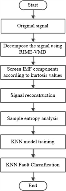
3.2. Diagnostic process

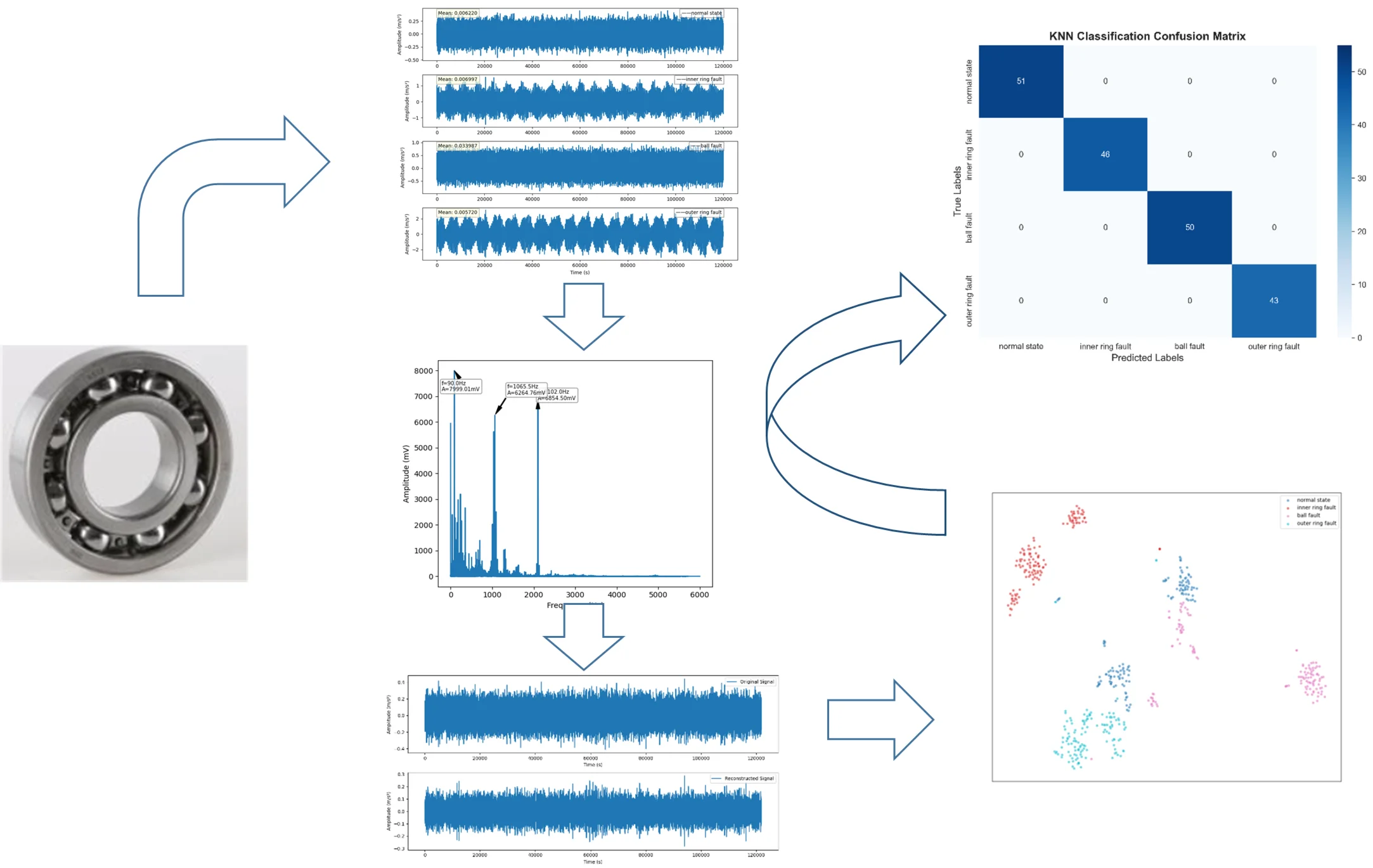
Bearing fault signals are nonlinear and non-stationary, and the fault analysis process is as follows: First, sensors are arranged in different directions of the rotor system to collect vibration data. Then, RIME-VMD is used to decompose the initial signal. The optimal IMF components rich in fault information are screened out according to the kurtosis value, and signal reconstruction is performed. The sample entropy of the reconstructed signal is calculated as a nonlinear fault feature. The reconstructed dataset is divided into a training set, a validation set, and a test set. The training set and validation set are used to train the KNN model, and the trained model is saved. Finally, the test set is used to evaluate the accuracy and generalization ability of the model to achieve rapid fault diagnosis of bearing faults. The process is shown in Fig. 2.

Fig. 1Flow chart of RIME optimized VMD

Fig. 2Diagnostic flow chart

3.3. Fault diagnosis analysis

1) Data collection. The data in this study was sourced from the Electrical Engineering Laboratory of Case Western Reserve University. The SKF6205 deep groove roller bearing was selected as the research object. This bearing was equipped with 9 rollers, and its fault characteristics were simulated by a preset damage with a diameter of 0.1778 mm. The experiment was driven by a 2-horsepower motor, operating under a stable rotational speed of 1750 r/min. The bearing vibration signals were captured in real time at a high-frequency sampling rate of 12 kHz, forming a time-series sample of 2048 data points for each collection. The study covered four typical states of the bearing: normal operation, inner ring fault, ball fault, and outer ring fault. Through systematic signal collection, a multi-dimensional fault feature database was constructed, providing accurate and reliable data support for subsequent model training and performance verification.

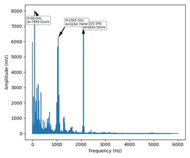
2) Analysis of original time series signals. The time-domain and frequency-domain representations of signals in four different states are shown in Fig. 3 and Fig. 4.

Fig. 3Original time series of the four states

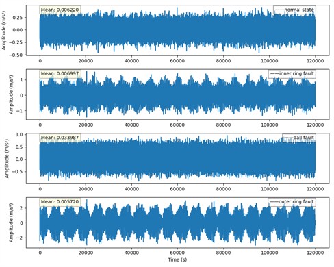
The figure shows the original time-series signals of rolling bearings in four states (normal, inner ring fault, ball fault, and outer ring fault). In terms of time-series signals, although each state has differences in fluctuation characteristics, the boundaries between different states are blurred and difficult to distinguish intuitively due to the complexity of the signals and noise interference. In the frequency-domain diagrams, the frequency distributions of different fault states overlap, making it difficult to accurately determine the characteristic frequencies. Since it is difficult to effectively distinguish each state based solely on these two types of diagrams, feature extraction methods based on intelligent algorithms, such as optimized decomposition algorithms like RIME-VMD, need to be adopted to deeply excavate the hidden features of the signals, improve the accuracy of judging the operating status and fault types of rolling bearings, and provide more reliable support for fault diagnosis and equipment maintenance.

3) Decomposition and reconstruction of signals. In the field of signal decomposition, the RIME-VMD, GA-VMD, GWO-VMD and AOA-VMD methods were tested and compared, showing different performance due to differences in the setting of their parameters $\left[K,\alpha \right]$. The decomposition mode number $K$ controls the fineness of signal deconstruction: a too small value is prone to missing key features, while a too large value causes over-decomposition. The penalty factor $\alpha$ coordinates decomposition accuracy and smoothness, and improper values will lead to signal distortion or detail loss. To accurately explore the influence of parameters, the search interval of $K$ was set to [2, 10], and the range of $\alpha$ was set to [100, 2500]. After $T$ iterations of trial and error, each algorithm screened out the optimal parameter strategy. Among them, the RIME algorithm, relying on a unique optimization mechanism, finally determined $\left(K,\alpha \right)=$ (9, 400) as the best parameter combination, which can effectively capture the multi-scale features of the signal under this configuration. The GA-VMD method set the parameter combination as $\left(K,\alpha \right)$ = (9, 1600) through experience and experiments, balancing the integrity of signal decomposition and detail retention. The GWO-VMD algorithm found the parameter solution of $\left(K,\alpha \right)$ = (8, 2000), achieving a balance between signal smoothness and accuracy with a larger penalty factor $\alpha$. The AOA-VMD algorithm, leveraging its swarm intelligence optimization characteristics, identified $\left(K,\alpha \right)$ = (8, 1900) as the suitable parameter combination, and achieved a balance between decomposition accuracy and detail capture. These parameter settings provide a specific reference for the comparison of signal decomposition effects of the three methods. Taking the inner race fault as an example, a data sample of 500 points was selected, and the signal decomposition is shown in Fig. 5.

Fig. 4Frequency-domain display of four states

a) Normal state

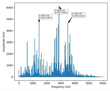
b) Inner ring fault

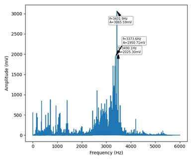
c) Ball fault

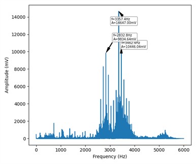
d) Outer ring fault

As shown in Fig. 5, each method decomposes the original signal into multiple sub-signals. These sub-signals exhibit very similar time-domain and frequency-domain characteristics, showing no obvious differences and containing identical or highly overlapping information, which leads to redundancy. Processing a large number of sub-signals increases the computational burden and reduces efficiency. Among them, over-decomposition occurs in the other three methods except RIME-VMD. Over-decomposition may mistake noise for important signal components, thereby amplifying the impact of noise. Therefore, further processing and analysis of the decomposed sub-signals are required to remove redundant information and noise and extract useful features. To further compare the advantages and disadvantages of the three algorithms, an iterative graph analysis can be performed, as shown in Fig. 6.

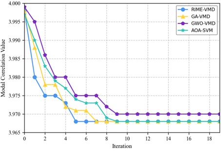
As shown in Fig. 6, in the initial several iterations, the median values of all algorithms show a significant downward trend, indicating that they are all rapidly converging to the optimal solution. The RIME-VMD algorithm descends the fastest in the first few iterations, demonstrating the fastest convergence speed. After approximately the 9th iteration, the median values of all algorithms tend to stabilize with minimal variation, suggesting that each algorithm has approached or reached a local optimal solution. At the end of 18 iterations, the RIME-VMD algorithm achieves the lowest median value. Overall, the RIME-VMD algorithm performs best in both convergence speed and final results.

Fig. 5Signal decomposition

Fig. 6Iterative diagram for algorithm comparison

The Pearson Correlation Coefficient (PCC) is a statistic used to measure the linear correlation degree between two continuous variables, with its value range between –1 and 1. The method combining the Pearson Correlation Coefficient (PCC) with the IMF components has demonstrated significant advantages. The PCC value between each IMF component and the fault state is calculated to quantify their linear correlation. The closer the PCC value is to 1 or –1, the stronger the correlation between the IMF component and the fault state, thereby screening out the key components reflecting fault characteristics. This method can not only accurately locate the fault source but also effectively separate the noise and fault features in the signal, improving the accuracy of diagnosis. The relationship between the magnitude of the PCC value and the linear relationship between the two variables is shown in Table 1.

The correlation coefficients of each IMF component are calculated using PCC, and the calculation results are shown in Table 2.

In all states, the PCC coefficients of IMF3 and IMF5 are generally high, indicating that these IMF components contain more fault characteristic information. For each IMF combination, signal reconstruction was performed, followed by classifying signals under different states using the same classification model. Table 3 presents the classification accuracy corresponding to different IMF combinations, from which it could be observed that the combination of IMF3 and IMF5 was more reasonable.

To evaluate the stability of PCC selection under different noise levels, noises of varying intensities (specifically low, medium, and high noise levels) were added to the original signal by setting different noise variances. Table 4 presents the performance of PCC coefficients for each IMF component under different noise levels. It can be observed from the table that the PCC coefficients of IMF3 and IMF5 consistently maintain relatively high values across different scenarios (low, medium, and high noise). This indicates that selecting IMF3 and IMF5 via PCC for signal reconstruction exhibits good stability when confronted with different noise interferences.

These two components were selected for signal reconstruction to effectively extract and retain key fault characteristic information in the signal, while removing noise and other irrelevant signal components. The reconstructed signal is shown in Fig. 7.

Fig. 7Reconstructed signals

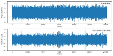
a) Original and reconstructed signals in normal state

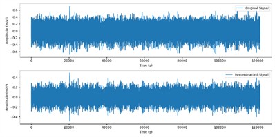
b) Original and reconstructed signals in inner ring fault state

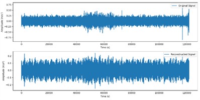
c) Original and reconstructed signals in ball fault state

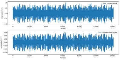
d) Original and reconstructed signals in outer ring fault state

4) Fault Diagnosis Analysis. Fig. 8 shows the visualization results of multi-scale sample entropy using RIME-VMD, GA-VMD, GWO-VMD and AOA-VMD methods, all of which use t-SNE dimensionality reduction technology to project multi-dimensional data onto a two-dimensional plane. In Fig. 8(b), although the signal reconstructed by the GA-VMD method can distinguish different states to a certain extent, some categories overlap, leading to unclear classification. The same applies to GWO-VMD in Fig. 8(c) and AOA-VMD in Fig. 8(d). In contrast, the signal reconstructed by the RIME-VMD method in Fig. 8(a) shows more compact distribution and higher separation of points in each category, with significantly reduced overlapping. It can be seen that the RIME-VMD method can more clearly distinguish different states when reconstructing signals, reducing classification uncertainty, which is superior to the GA-VMD, GWO-VMD and AOA-VMD methods. This is of great significance for fields such as fault diagnosis and condition monitoring, as it helps to more accurately identify the status of equipment and potential problems.

Fig. 8Visualization of multi-scale sample entropy

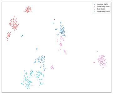
a) RIME-VMD reconstructed signal

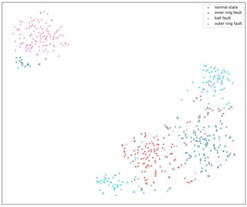
b) GA-VMD reconstructed signal

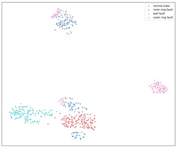
c) GWO-VMD reconstructed signal

d) AOA-VMD reconstructed signal

To further measure the accuracy of several methods, 100 time windows were selected for each modal component of the four states to extract multi-scale sample entropy, resulting in 100×20 training samples. Finally, 400×20 samples of the four states were labeled and used as inputs to the KNN classifier. The results are shown in Fig. 9.

It can be seen from Fig. 9 that the GA-VMD, GWO-VMD and AOA-VMD methods can predict fault categories well for most categories, but there are certain deviations between the predicted values and the true values for individual categories. In contrast, the identification results of RIME-VMD show higher overall accuracy and stability. Although there are also some deviations in the results of RIME-VMD, these deviations are smaller than those of the other three methods, and the distribution is more concentrated. Especially for some key categories, the predicted values of RIME-VMD almost completely coincide with the true values, demonstrating its superior performance in fault identification.

Fig. 9KNN classification confusion matrix

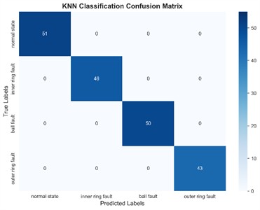
a) RIME-VMD

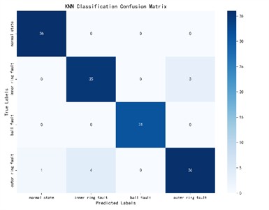
b) GA-VMD

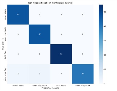
c) GWO-VMD

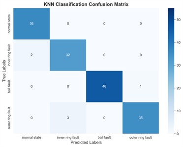
d) AOA-VMD

To evaluate the stability and significance of the RIME-VMD method, validation was conducted using a “multiple random partitioning + cross-validation” approach, with the following steps:

(1) Data partitioning: Divide all data into five equal parts.

(2) Cyclic Evaluation:

– Use the first sample as the test set and the remaining four samples as the training set, then calculate the metric once.

– Use the second sample as the test set and the remaining four samples as the training set, then recalculate the metrics.

– Repeat the above steps until all 5 portions have served as the test set, yielding 5 sets of metrics.

(3) Statistical Results: The calculated averages are summarized in tabular form. See Table 5 for details.

In summary, we can conclude that the RIME-VMD method is superior to the GA-VMD, GWO-VMD and AOA-VMD methods in fault identification. Especially when dealing with complex and changeable fault data, RIME-VMD can provide more accurate and reliable prediction results. This finding is of great significance for practical engineering applications and helps to improve the efficiency of equipment fault diagnosis and maintenance.

To further verify the method proposed in this paper, a Data Combination test was conducted. The bearing load was set to 2 horsepower, and the damage diameters were 0.1778 mm, 0.3556 mm, 0.5334 mm, and 0.7112 mm respectively; tests and analyses were carried out for these four operating states. Each Intrinsic Mode Function (IMF) under each state was constructed into a 100×20 training sample. Finally, a total of 400×20 samples from the four states were labeled and input into SVM and KNN classifiers respectively. As can be seen from Table 6, the test results show that there were a small number of sample misclassifications when using SVM, while the accuracy rate of the KNN comprehensive judgment method reached 100 %.

3.4. Verification of real-time performance

To verify the real-time performance of the proposed method, experiments were designed from three aspects: processing delay, computational efficiency, and adaptability to embedded/edge computing. The experimental platforms and parameter settings are as follows:

Experimental Platforms: General-purpose computing platform: Intel i7-12700H CPU, 16GB DDR4 memory, Windows 11 operating system; Edge computing platform: Raspberry Pi 4B (4-core ARM Cortex-A72 CPU, 4GB LPDDR4 memory).

Experimental Parameters: The bearing fault dataset from the “data combination” was adopted, which has a load of 2 horsepower and a damage diameter range of 0.1778-0.7112 mm; Sample size: 400×20.

Each platform was run independently for 10 experiments, and the average value and standard deviation were calculated for final results.

1) Analysis of processing delay. Table 7 presents the comparison of processing delays across different platforms.

As can be seen from the table, on the general-purpose computing platform, the average delay of RIME-VMD in processing 400×20 samples is 18.3 ms with a standard deviation of 1.5 ms, both of which are lower than the corresponding values of the other three methods. This indicates that the proposed method has better real-time performance on general-purpose devices.

On the edge computing platform, the average delay of RIME-VMD is 69.5 ms, which is not only lower than the requirement threshold of “delay < 100 ms” for industrial real-time diagnosis but also lower than that of the other three methods. This proves that the proposed method still has real-time processing capability on edge devices.

2) Analysis of Computational Efficiency. The computational efficiency is analyzed from two aspects: “Samples Processed Per Second (SPS)” and “Resource Utilization”, with specific details shown in Table 8.

Efficiency: On the Raspberry Pi 4B, the SPS (Samples Processed Per Second) of the proposed method is 5.7 (i.e., processing 5.7 sets of 100×20 samples per second), which is 1.8 times that of GA-VMD. This indicates that the proposed method has higher throughput and can cope with scenarios with higher-frequency data input.

Resource Occupancy: During processing, the proposed method has an average CPU utilization rate of 38 % and a peak memory occupancy of 46 MB. In contrast, GA-VMD has a CPU utilization rate of 63 % and a memory occupancy of 89 MB. This proves that the proposed method has lower hardware resource requirements and is more suitable for resource-constrained environments.

3) Feasibility Conclusion for Embedded/Edge Computing. Based on the above data, RIME-VMD can operate stably on edge devices, with the following key performance indicators meeting application requirements: The processing delay satisfies industrial real-time demands (i.e., < 100 ms); Its resource occupancy is lower than that of the other three methods, requiring no high-performance hardware support and thus being adaptable to low-cost embedded devices.

Therefore, RIME-VMD is feasible for embedded/edge computing scenarios and can be applied to on-site real-time fault diagnosis.

3.5. Verification of generalization ability

To comprehensively evaluate the generalization ability of the model, on the basis of verification using the CWRU dataset, the XJTU-SY dataset (Xi'an Jiaotong University - Shaoxing University of Arts and Sciences Bearing Dataset) was supplemented. This dataset covers “full-life cycle faults” (ranging from normal conditions to early-stage, mid-stage, and late-stage faults) and includes operating conditions with variable rotational speeds (1000-3000 r/min) and variable loads (0-3000 N). In contrast to the fixed operating conditions of the CWRU dataset, it is used to test the model's generalization ability under varying operating conditions.

After the simulation model is trained in the benchmark scenario, it is migrated to a similar but distinct laboratory scenario to verify its generalization ability across different operating conditions. The normal/single-fault samples from the CWRU dataset are used as the training set (divided according to the original proportion, with 70 % allocated for training), while the full-life cycle fault samples from the XJTU-SY dataset serve as the test set (100 % used for testing, with no training data included). The accuracy of the original study, which was based on training with the CWRU dataset and subsequent testing with the same dataset (CWRU training → CWRU testing), is retained as the benchmark. Additionally, the accuracies of GA-VMD, GWO-VMD, and AOA-VMD under the same cross-dataset testing are newly incorporated. The comparison of cross-dataset testing accuracies is presented in Table 9.

As can be seen from the table, when trained solely on the CWRU dataset, the model achieves an accuracy of only 85.3 % on the variable operating condition dataset. This is because the faults in the CWRU dataset occur under fixed operating conditions, while those in the XJTU-SY dataset occur under variable operating conditions – this discrepancy results in the model having weak ability to identify faults under variable operating conditions. After training with multi-source data, the accuracy on the variable operating condition dataset increases to 91.7 %. This indicates that by combining data from the CWRU and XJTU-SY datasets, the model learns more generalized fault features and reduces its reliance on the distribution of a single dataset. It can also be observed from the table that the RIME-VMD model has advantages over other models: its accuracy in composite fault testing is higher than that of other models. The reason lies in the attention module of this model, which can focus on the multi-fault features in composite faults, whereas other models are easily interfered with by redundant features. This thus verifies the generalization ability of RIME-VMD under varying operating conditions.