Abstract
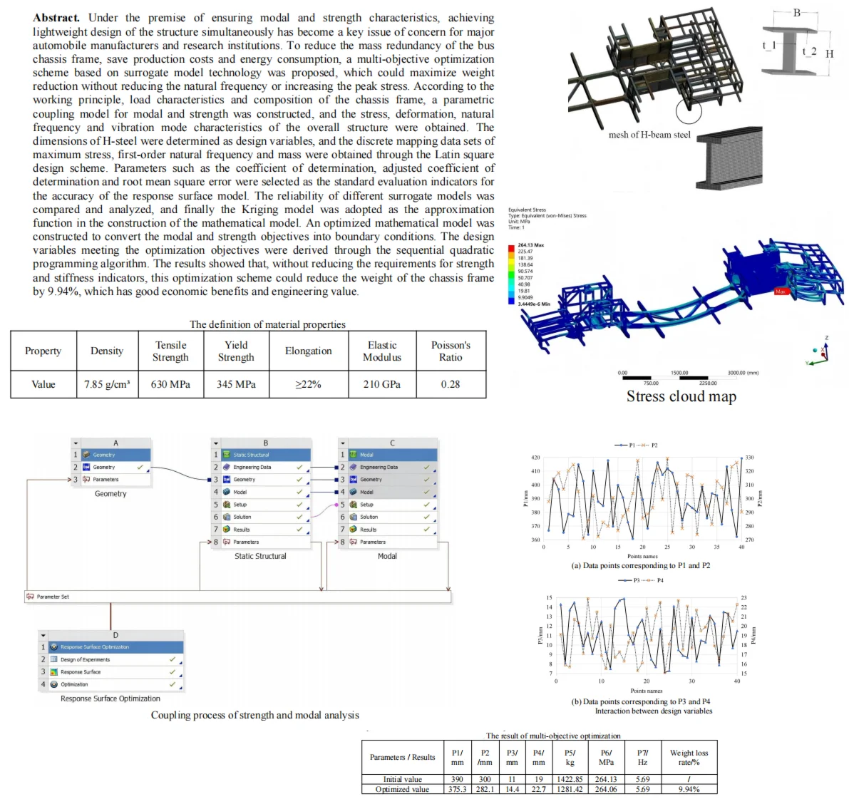
Under the premise of ensuring modal and strength characteristics, achieving lightweight design of the structure simultaneously has become a key issue of concern for major automobile manufacturers and research institutions. To reduce the mass redundancy of the bus chassis frame, save production costs and energy consumption, a multi-objective optimization scheme based on surrogate model technology was proposed, which could maximize weight reduction without reducing the natural frequency or increasing the peak stress. According to the working principle, load characteristics and composition of the chassis frame, a parametric coupling model for modal and strength was constructed, and the stress, deformation, natural frequency and vibration mode characteristics of the overall structure were obtained. The dimensions of H-steel were determined as design variables, and the discrete mapping data sets of maximum stress, first-order natural frequency and mass were obtained through the Latin square design scheme. Parameters such as the coefficient of determination, adjusted coefficient of determination and root mean square error were selected as the standard evaluation indicators for the accuracy of the response surface model. The reliability of different surrogate models was compared and analyzed, and finally the Kriging model was adopted as the approximation function in the construction of the mathematical model. An optimized mathematical model was constructed to convert the modal and strength objectives into boundary conditions. The design variables meeting the optimization objectives were derived through the sequential quadratic programming algorithm. The results showed that, without reducing the requirements for strength and stiffness indicators, this optimization scheme could reduce the weight of the chassis frame by 9.94 %, which has good economic benefits and engineering value.
Highlights
- To reduce the mass redundancy of the bus chassis frame, save production costs and energy consumption, a multi-objective optimization scheme based on surrogate model technology was proposed, which could maximize weight reduction without reducing the natural frequency or increasing the peak stress.
- According to the working principle, load characteristics and composition of the chassis frame, a parametric coupling model for modal and strength was constructed, and the stress, deformation, natural frequency and vibration mode characteristics of the overall structure were obtained.
- Response surface models for mass, peak stress, and first natural frequency were established respectively and verified through systematic error analysis.
1. Introduction
As a common means of long-distance passenger transportation, the safety and stability of buses are the key points in their structural design, especially for the crucial load-bearing component, the chassis frame [1]. The modal characteristics of the chassis frame are of critical importance. As a key load-bearing component of the bus, resonance is highly likely to occur if the natural modal frequency of the chassis frame aligns closely with the external excitation frequency. Furthermore, as the automotive industry increasingly prioritizes low-noise performance, modal optimization has become indispensable. When the excitation frequency caused by uneven road surfaces approaches a specific modal frequency of the frame, severe vibrations may arise. These vibrations not only compromise passenger comfort but also lead to fatigue damage in frame components over time, thereby reducing the service life of the frame. During full-load climbing, the frame must withstand significant longitudinal, vertical, and lateral forces. Insufficient frame strength can result in bending or even fracture, posing a serious threat to driving safety [2, 3]. Additionally, frequent starts and stops, turns, and sudden braking during vehicle operation impose dynamic loads on the frame, further testing its strength reserve. For buses, reducing weight effectively decreases the load and lowers power consumption. Through reasonable frame optimization design, weight reduction without compromising frame performance enhances the economic efficiency of bus operations. Moreover, with the growing adoption of electric vehicles in the bus sector, vehicle weight significantly impacts driving range. Reducing the frame's weight improves the driving range of electric buses, alleviates range anxiety, and promotes the further development of electric vehicles in the bus market. However, simple weight reduction may adversely affect the frame’s modal and strength properties. Ensuring that the frame's modal and strength characteristics meet performance requirements while achieving lightweighting remains a key challenge. Representative achievements in related research directions include: Daşdemir [4] conducted a simulation analysis of the modal characteristics of piezoelectric plates under specific conditions based on the finite element method, taking into account the stress state of the initial conditions, which belongs to an indirect coupling model. Mohammad [5] conducted strength analysis and weight reduction design on the structure of electric vehicles through the finite element method, which can verify the lightweight research scheme without increasing the load response. Talebitooti [6] conducted multi-objective optimization on the porous structure of the inner lining of the cylindrical shell, combined with the non-dominated sorting genetic algorithm, to reconfigure the porous structure and improve its mechanical properties. Celik [7] performed a structural strength analysis of a rotary mechanism using advanced computer-aided engineering (CAE) simulation techniques. The study effectively evaluated the load response under various operational conditions, thereby providing a critical foundation for structural optimization and design improvement. Snezana [8] performed a comprehensive strength analysis of the eight-wheel bogie in a bucket-wheel excavator with finite element method, proposed a targeted structural optimization scheme, and validated the accuracy and reliability of the finite element model through comparative analysis. Joo [9] applied finite element modal analysis and integrated it with multi-point input-multi-point output modal testing to investigate the inherent vibration characteristics of the system. Based on a thorough examination of excitation frequencies, a comprehensive optimization approach that combines size and topology optimization was developed. Nitalikar [10] employed finite element numerical simulations to examine how thickness variations affect guided wave propagation. The approach proved highly effective in accurately capturing geometric discontinuities and exhibited strong adaptability and precision in complex structural analyses.
Based on the working conditions of the bus chassis frame, it is evident that strength and stiffness criteria are essential in structural optimization design [11]. Neglecting these factors may result in traditional single-objective optimization schemes failing to fully satisfy reliability requirements [12]. Therefore, a lightweight approach based on multi-objective optimization is proposed, enabling the achievement of an improved structural design without compromising performance – indeed, potentially enhancing it. Compared with previous studies, the main innovation points of this study are as follows: (1) A coupled modal-strength analysis model was introduced, which breaks the limitation of previous studies that typically treated modal analysis and strength analysis as independent processes. Unlike existing research, the proposed coupled model can not only accurately obtain the peak stress values and natural frequencies of the structure but also realize the simultaneous parameterization of design variables, achieving the integrated analysis of dynamic performance and mechanical strength that was lacking in prior works. (2) Response surface models for mass, peak stress, and first natural frequency were established respectively and verified through systematic error analysis. This makes up for the shortcomings of previous studies where response surface models were often single-target (e.g., only focusing on stress or mass) or lacked rigorous error verification. The models established in this study not only comprehensively cover key performance indicators but also ensure accuracy through error analysis, which helps to efficiently determine the optimal design variables under various constraints. Compared with the inefficient trial-and-error optimization methods in traditional research, this significantly improves the optimization effect and effectively reduces research and application costs.
2. Modal and strength analysis of the chassis frame
2.1. Establishment of the finite element model
The position of the bus chassis frame is shown in Fig. 1(a). According to the structural principle of the chassis frame, it is known that its external dimensions, the connection structure of each component, and other geometric features have a crucial impact on dynamic performance. For instance, the beam structure size of the chassis frame, any dimensional deviation will lead to errors in its load-bearing capacity calculation. Details such as installation holes and reinforcing ribs must also be accurately modeled. Although these details are small, they may play a significant role in local stress distribution and affect the reliability of the overall structure. The connection methods among the components of the chassis frame are diverse, such as welding and bolt connection. For welding connections, they can be regarded as rigid connections. During modeling, it is necessary to ensure the correct constraint of the degrees of freedom at the connection nodes to simulate their integrity. Bolt connections are relatively complex and require consideration of the preload of the bolts, the contact relationship between the bolts and the connected parts, etc. Only by reasonably simulating the connection relationship can the force transmission and cooperative working conditions among the components of the chassis frame under load be truly reflected.
Fig. 1Model of chassis frame
a) The position of the chassis frame
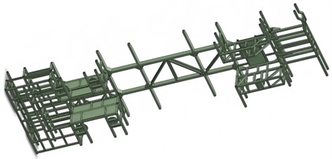
b) The simplified model of chassis frame
To ensure the accuracy and efficiency of finite element analysis, it is necessary to carry out effective simplification processing on the model. The geometric features that have a significant impact on the mechanical performance and modal results of the frame should be retained. Features such as chamfers and small holes that are subject to high stress concentration, if ignored, may lead to incorrect stress distribution calculations, as these areas are often the starting points of structural failure. However, minor features that have a negligible impact on the analysis results, such as slight casting marks, non-critical minor protrusions or depressions, can be deleted without affecting the overall mechanical behavior. For components in the chassis frame that have complex shapes but relatively simple mechanical properties, reasonable simplification can be carried out. For instance, some irregularly shaped reinforcing plates, if their main function is to enhance local rigidity, can be simplified into regular shapes, such as rectangles or circles. During simplification, it is necessary to ensure that the key mechanical characteristics of the simplified structure are similar to those of the original structure, such as keeping the area, moment of inertia and other parameters as consistent as possible, so as to maintain their equivalent influence on the overall performance of the frame. The geometric shape of the chassis frame is constructed in Solidworks, as shown in Fig. 1(b).
The chassis frame must bear the weight of the vehicle itself, passengers and cargo, as well as various dynamic loads during driving, such as forces generated during acceleration, braking and turning. The material must have sufficient strength to prevent fractures under normal use and extreme conditions. The chassis frame needs to maintain a certain rigidity to avoid excessive deformation under force. Excessive deformation will affect the vehicle’s handling stability, comfort and the normal operation of components. The prices of different materials vary greatly. Under the premise of meeting the vehicle's performance requirements, materials with appropriate costs should be selected. The vehicle's driving environment is complex, and the chassis frame is exposed to the outside for a long time, making it vulnerable to erosion by rain, moisture and salt. Based on the above requirements, Q345 high-strength alloy steel with good comprehensive performance is selected, of which material properties is shown in Table 1, which can meet the requirements of the vehicle under complex conditions.
Table 1The definition of material properties
Property | Density | Tensile strength | Yield strength | Elongation | Elastic modulus | Poisson’s ratio |
Value | 7.85 g/cm3 | 630 MPa | 345 MPa | ≥ 22 % | 210 GPa | 0.28 |
2.2. Preprocessing of the coupling model
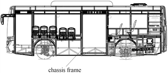
To ensure the reliability of the dynamic characteristic optimization of the chassis frame, a coupled model integrating modal and strength analysis is employed, as illustrated in Fig. 2. This coupled analysis facilitates the identification of structural weak points under the combined effects of static and dynamic loads, thereby providing critical data for multi-objective optimization. During modal analysis, it is observed that specific regions of the structure exhibit significant vibration at certain modes, while these regions are already subjected to high stress during static analysis. The coupled analysis enables a comprehensive assessment of the safety and reliability of the structure under such conditions. Based on the findings from the coupled analysis, targeted structural optimization can be performed to enhance performance, mitigate failure risks, and simultaneously minimize material usage for lightweight design [13].
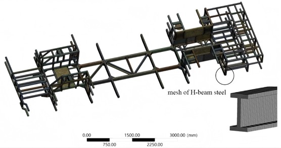
Meshing is a critical step to ensure the accuracy of finite element analysis. For chassis frames, complex geometries require finer meshes to capture detailed structural behavior. Mesh refinement should be applied at locations such as holes and corners where stress concentrations occur, as these regions demand sufficient resolution to accurately represent stress variations. For simple geometries, such as regular rectangular prisms, coarser meshes can be used without compromising accuracy. The dimensions of each side of an element should ideally be approximately equal, with the aspect ratio approaching 1 for optimal performance. In thin plate structure analysis involving quadrilateral elements, an excessively high aspect ratio may result in unreasonable deformations under load, thereby reducing calculation accuracy. It is generally recommended that the aspect ratio in structural analysis does not exceed 5-10. The transition of mesh size within the model should be gradual to avoid abrupt changes. Sudden variations in mesh size between adjacent regions can lead to numerical oscillations during computation, which may compromise the accuracy of the results [14]. When transitioning from coarse to fine mesh regions, a smooth size change rate of approximately 1.5-2 is typically considered appropriate. Based on the structure of the chassis model, take 1/20 of the characteristic dimension. At the same time, set the “Relevance Center” and select Medium to adjust the overall mesh density. Also, set parameters such as “Transition” and “Smoothing” to make the mesh transition more uniform. Through local mesh optimization, the final mesh division result is shown in Fig. 5.
Fig. 2Coupling process of strength and modal analysis
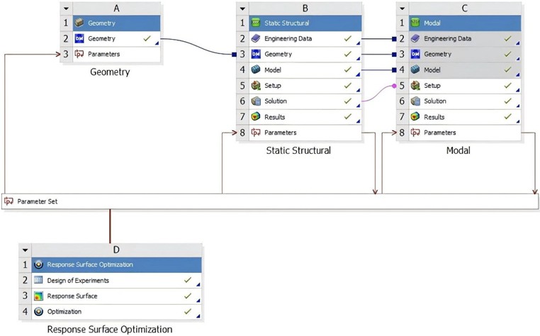
Fig. 3The mesh of the finite element model
In Workbench, Orthogonal Quality and Aspect Ratio are two core indicators for evaluating mesh quality, which directly affect the accuracy and convergence of finite element analysis results, as shown in Fig. 4. It can be seen that the mesh quality meets the calculation requirements. Orthogonal Quality focuses on the regularity of the element shape and directly affects the accuracy of stress calculation. Low-quality elements need to be optimized first. Aspect Ratio focuses on the elongation of the element and has a greater impact on the convergence of the calculation. A reasonable threshold should be set according to the analysis type. In the chassis analysis, both need to be checked in combination. Key areas (such as the connection points of the frame longitudinal beams and cross beams) need to simultaneously meet Orthogonal Quality ≥ 0.6 and Aspect Ratio ≤ 3 to ensure reliable results.
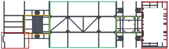
The main load-bearing areas of the chassis frame are shown in Fig. 5. It can be seen that there is an obvious imbalance and asymmetry in the load distribution. For the connection between different components, bonding constraint is employed to simulate welding and bolted joints. The nodes on the contact surface share identical displacements and prohibits any relative sliding or separation. Given the primary focus on the overall force and deformation of the frame, with less stringent requirements for local details at the bolted connections, the components in the bolted connection regions can be modeled as bonded contact and analyzed as a rigid assembly. This simplification not only significantly improves computational efficiency but also enables rapid acquisition of the overall mechanical response of the frame. The H-beam is composed of a vertical web and two horizontal flanges symmetrically positioned on either side of the web. This distinctive configuration confers superior structural mechanical properties compared to other steel profiles. The inner and outer surfaces of the flanges are typically parallel, providing a flat and regular contact surface for connections with other components via welding, bolting, or riveting. This design facilitates construction operations while ensuring the stability and reliability of the connection. Additionally, the relatively wide flanges maintain consistent thickness from root to tip, enhancing the out-of-plane stability of the steel beam and improving its overall torsional resistance. The web primarily withstands the shear force acting on the beam. With a relatively thin web thickness, this design reduces material usage without compromising structural load-bearing capacity, thereby lowering the self-weight of the structure and optimizing material efficiency.
Fig. 4The evaluation results of the finite element mesh
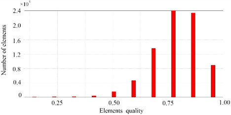
a) The maximum orthogonal quality
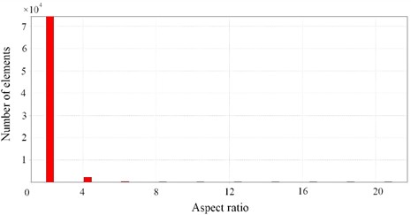
b) The maximum aspect ratio
Fig. 5The main load-bearing area
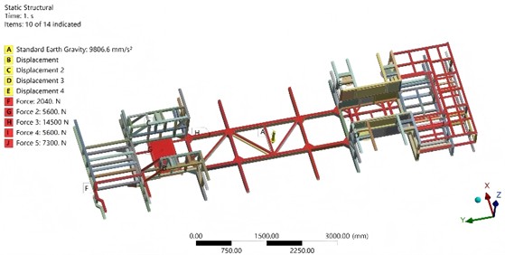
Under the extreme load conditions, the load and constraints of the chassis frame are set as shown in Fig. 6. The wheel transmits road forces to the frame via the suspension system. In static analysis, two primary load types are considered: the supporting force exerted by the suspension on the frame and the vertical impact force. To simulate the supporting force under flat road conditions, a vertical concentrated or distributed load can be applied at the connection points between the frame and the suspension. For the impact force, an empirically determined large instantaneous concentrated force may be applied, while constraining the remaining degrees of freedom at the suspension attachment points to reflect the suspension’s restraining effect on the frame. Additionally, centrifugal force generates lateral loads on the frame during vehicle turns. The magnitude of this force can be calculated based on the turning radius, driving speed, and total vehicle mass. It is typically applied as a lateral concentrated or distributed force acting at the height of the center of gravity, directed outward along the turning radius.
Fig. 6The setting of load and convenient conditions
2.3. Modal analysis
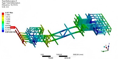
The first six mode shape analysis results of the chassis frame can be obtained through finite element calculation, as shown in Fig. 7. The first-order mode corresponds to torsional vibration along the horizontal direction, which induces longitudinal torsion in the bus. During this mode, the entire chassis frame rotates about an axis perpendicular to its base plane and the natural frequency is 5.69 Hz. The ends of the frame twist in opposite directions, while the central region experiences minimal torsional displacement. The second-order mode manifests as vertical bending vibration, where the chassis frame deforms in a manner similar to a simply supported beam. The maximum bending deformation occurs at the center, with relatively smaller deformations at both ends. The third-order mode involves transverse bending vibration; the frame bends laterally, with the central section acting as a nodal point and the two sides bending in opposite directions. The fourth-order mode represents second-order torsion, which is more complex than the first-order torsion. It features multiple torsional centers, with significant variations in torsional angles and directions across different parts of the frame. The fifth-order mode refers to second-order bending, characterized by a more complex transverse bending pattern. This may include multiple peaks and troughs in the bending shape, resulting in a more intricate deformation profile. The sixth-order mode is a composite mode combining both bending and torsional vibrations, where various types of vibration occur simultaneously at different locations across the chassis.
To verify the reliability of the finite element model, the natural frequencies were tested and validated for the free modal conditions, as shown in Fig. 8. The frame was struck with a force hammer to generate transient excitation. Under the excitation, the frame vibrated freely, and the vibration response signals were collected using an acceleration sensor to identify the natural frequencies of the frame. The test and comparison results are shown in Table 2. It can be seen that the maximum deviation of the first six natural frequencies is only 5.1 %, which indicates that the finite element model has high accuracy.
Fig. 7The first six modal shapes
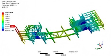
a) The first order
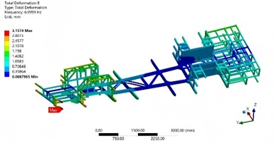
b) The second order
c) The third order
d) The fourth order
e) The fifth order
f) The sixth order
Fig. 8Test of natural frequency in free modal
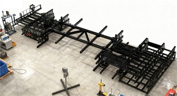
Table 2The test and comparison results of natural frequency
Order | 1 | 2 | 3 | 4 | 5 | 6 |
Simulation value / Hz | 2.25 | 2.89 | 3.37 | 4.46 | 4.99 | 6.62 |
Test value / Hz | 2.37 | 2.95 | 3.44 | 4.55 | 5.07 | 6.74 |
2.4. Strength analysis
The strength analysis results of the chassis frame obtained through finite element analysis are shown in Fig. 9. It can be seen that the stress distribution of the chassis frame shows obvious regional differences. Generally, the stress is mainly concentrated in the key connection points and areas that bear the main load. The connection points between the frame and the axle, the suspension mounting points, and other areas, due to the need to withstand complex loads during vehicle operation, including vertical loads, horizontal loads, and torque, have relatively high stress values. In contrast, in some non-critical structural areas of the chassis frame, such as the middle parts of some crossbeams, the stress values are relatively low. After analysis, it is determined that the maximum stress value of the chassis frame is 264.13 MPa, and this maximum stress occurs near the connection between the left front suspension and the frame. The reason for the stress concentration at this location is mainly that this area not only has to bear the vertical impact force from the road surface during vehicle operation but also has to transfer the lateral and longitudinal forces generated by the suspension system during steering and braking. The superposition of multiple loads causes the stress at this location to be much higher than that in other areas. Compared with the material's yield strength of 345 MPa, there is a considerable safety margin, which also reflects the necessity of lightweight design. The maximum deformation of the chassis frame is 4.23 mm, occurring at the mid-span position of the middle crossbeam of the frame. This position, during vehicle operation, due to the action of vertical loads, is similar to a simply supported beam structure, where the middle part bears the maximum bending moment and thus has the maximum deformation. Compared with the design deformation requirements of the chassis frame, the current maximum deformation is within the acceptable range.
Fig. 9Strength analysis results
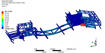
a) Stress cloud map
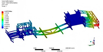
b) Displacement cloud map
3. Multi objective optimization and performance evaluation
3.1. Design of discrete samples
The parameterization of the model is one of the key steps in multi-objective optimization [15, 16]. The design variables are selected as the key cross-sectional geometric parameters of H-shaped steel, including: flange width , cross-sectional height , web thickness , and flange thickness , as shown in Fig. 10. These parameters directly determine the cross-sectional dimension characteristics of H-shaped steel and will affect the mass and mechanical properties of the structure (such as peak stress, natural frequency, etc.), which are the core variables in structural optimization design. In accordance with the provisions and requirements of the standard code GB/T 11263-2024, the value range of the parameterized dimensions is shown in Table 3. The overall structure is driven by the skeleton model, and the frame is divided into modules such as longitudinal beams, transverse beams, and connecting brackets, each of which is created through parameterized features. The Creo model is imported into Ansys Workbench, and the geometric parameters are identified using the Design Modeler module and marked as parameter variables. Adjustable ranges are set for key parameters for subsequent optimization [16].
Fig. 10Definition of parametric dimensions
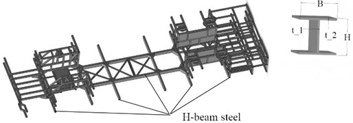
Table 3The range of values for design variables
Name of parameter | Code | Initial value / mm | Minimum value / mm | Maximum value / mm |
P1 | 390 | 360 | 420 | |
P2 | 300 | 270 | 330 | |
P3 | 11 | 7 | 15 | |
P4 | 19 | 15 | 23 |
Table 4Discrete sample data
Number | P1 / mm | P2 / mm | P3 / mm | P4 / mm | P5 / kg | P6 / MPa | P7 / Hz |
1 | 366.75 | 297.75 | 14.3 | 19.1 | 1079.42 | 258.52 | 5.10 |
2 | 404.25 | 314.25 | 8.1 | 15.9 | 1084.53 | 178.22 | 7.24 |
3 | 396.75 | 318.75 | 13.7 | 15.7 | 1202.47 | 208.98 | 6.49 |
4 | 365.25 | 306.75 | 14.5 | 20.7 | 1212.34 | 267.70 | 4.82 |
5 | 378.75 | 320.25 | 12.1 | 20.3 | 1231.86 | 239.05 | 5.54 |
6 | 377.25 | 324.75 | 9.9 | 17.1 | 1257.40 | 198.49 | 6.90 |
7 | 414.75 | 305.25 | 11.3 | 22.9 | 1283.72 | 256.36 | 4.51 |
8 | 402.75 | 270.75 | 9.1 | 18.7 | 1289.71 | 223.52 | 5.81 |
9 | 363.75 | 284.25 | 10.9 | 21.5 | 1342.81 | 267.44 | 4.86 |
10 | 410.25 | 302.25 | 12.5 | 16.9 | 1400.73 | 212.33 | 6.19 |
11 | 387.75 | 272.25 | 9.3 | 15.5 | 1406.43 | 198.52 | 7.20 |
12 | 384.75 | 282.75 | 7.5 | 20.1 | 1407.64 | 232.83 | 5.19 |
13 | 417.75 | 279.75 | 13.9 | 16.7 | 1423.57 | 227.40 | 5.73 |
14 | 369.75 | 300.75 | 14.7 | 17.3 | 1426.29 | 245.57 | 5.86 |
15 | 399.75 | 276.75 | 14.9 | 16.3 | 1428.37 | 242.13 | 5.71 |
16 | 390.75 | 287.25 | 11.1 | 18.3 | 1429.25 | 227.93 | 5.46 |
17 | 372.75 | 291.75 | 10.1 | 19.3 | 1457.14 | 235.54 | 5.35 |
18 | 360.75 | 303.75 | 11.9 | 15.3 | 1467.95 | 208.20 | 6.79 |
19 | 405.75 | 327.75 | 12.7 | 16.1 | 1482.69 | 198.65 | 6.38 |
20 | 389.25 | 285.75 | 10.7 | 21.9 | 1488.91 | 261.14 | 4.64 |
21 | 368.25 | 288.75 | 8.5 | 18.5 | 1501.21 | 223.28 | 5.69 |
22 | 401.25 | 293.25 | 7.7 | 21.1 | 1505.40 | 233.71 | 5.04 |
23 | 416.25 | 321.75 | 11.7 | 22.5 | 1534.50 | 247.16 | 4.56 |
24 | 407.25 | 299.25 | 7.1 | 15.1 | 1544.42 | 170.46 | 8.22 |
25 | 411.75 | 329.25 | 7.3 | 18.1 | 1551.36 | 190.19 | 6.47 |
26 | 408.75 | 275.25 | 14.1 | 19.7 | 1566.61 | 257.25 | 5.16 |
27 | 395.25 | 311.25 | 9.5 | 22.7 | 1590.34 | 251.71 | 4.74 |
28 | 374.25 | 278.25 | 8.9 | 17.5 | 1592.44 | 217.57 | 5.79 |
29 | 386.25 | 317.25 | 8.7 | 22.1 | 1608.9 | 243.26 | 5.46 |
30 | 383.25 | 315.75 | 12.9 | 17.7 | 1615.58 | 222.73 | 6.04 |
31 | 380.25 | 273.75 | 8.3 | 21.7 | 1627.28 | 257.79 | 4.80 |
32 | 398.25 | 309.75 | 10.5 | 19.5 | 1641.91 | 230.77 | 4.60 |
33 | 375.75 | 294.75 | 10.3 | 19.9 | 1701.60 | 240.06 | 5.20 |
34 | 393.75 | 281.25 | 13.1 | 20.9 | 1712.74 | 264.31 | 4.73 |
35 | 392.25 | 312.75 | 12.3 | 17.9 | 1731.64 | 219.05 | 5.78 |
36 | 371.25 | 308.25 | 7.9 | 16.5 | 1748.40 | 191.83 | 7.04 |
37 | 413.25 | 296.25 | 13.5 | 18.9 | 1755.34 | 236.28 | 5.05 |
38 | 381.75 | 323.25 | 13.3 | 21.3 | 1837.24 | 251.56 | 5.21 |
39 | 362.25 | 326.25 | 9.7 | 20.5 | 1852.57 | 231.47 | 5.86 |
40 | 419.25 | 290.25 | 11.5 | 22.3 | 1916.46 | 255.60 | 4.51 |
To enhance the strength and rigidity of the chassis frame, based on the results of modal and strength analysis, the optimization objectives are set as the minimum value of the mass P5, the minimum value of the maximum stress P6, and the maximum value of the first natural frequency P7. Considering the characteristics of the range of design variable values, the G-optimal central composite design method is adopted in this paper to generate the required sample data. During the continuous data exchange and iteration between ANSYS and Creo, the real-time sharing of parameter variables is achieved, thereby clarifying the optimization objectives corresponding to each design variable. Latin square design is particularly suitable for experimental scenarios involving two blocking factors (row and column factors) where the number of levels for each factor is identical. In the context of chassis frame optimization, when multiple design variables – such as the cross-sectional height of steel, flange width, and others – must be considered simultaneously, and external interfering factors need to be controlled, the Latin square design offers an effective approach to organize experiments systematically. This method enables the acquisition of critical experimental data with a minimal number of trials, thereby improving efficiency in the optimization process. Based on the Latin square design scheme, the specific results are shown in Table 4.
Based on the obtained discrete data table, a response surface model for optimization design can be further constructed. From the perspective of modeling, the selection of design points has a significant impact on the final results. If the number of design points is too large, it will prolong the optimization cycle and reduce the R&D efficiency. While if the number of design points is insufficient, it may lead to a decrease in the accuracy of the response surface model. Therefore, when constructing the response surface model, how to obtain a higher model accuracy with as few design points as possible becomes the key. In addition, Fig. 11 shows the correlation between each design variable. It can be seen that there is no overlap among the data points, indicating that all discrete data can effectively support the establishment of the response surface function.
Fig. 11Interaction between design variables
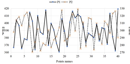
a) Data points corresponding to P1 and P2
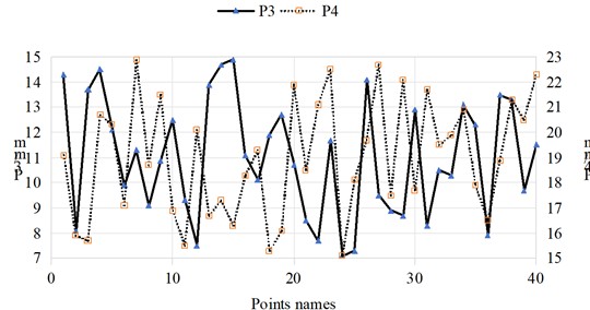
b) Data points corresponding to P3 and P4
3.2. Fitting and error analysis of response surface function
In the construction of response surface functions, Kriging model and quadratic polynomial model are two commonly used approximate modeling methods. They are based on different theoretical foundations and have significant differences in fitting characteristics and applicable scenarios. The core idea of the Kriging model is to interpolate based on the spatial correlation of sample points, and it describes the spatial correlation degree between sample points by constructing a variogram, thereby predicting the response values of unsampled points. It assumes that the spatial distribution of response values has randomness and structure, that is, the difference in response values between any two points is not only related to distance but also to spatial position. It has relatively flexible requirements for sample size, being able to handle both small and large sample scenarios, but the uniformity of the spatial distribution of sample points is more important. The quadratic polynomial model is a deterministic regression model that approximates the relationship between design variables and response values by fitting a quadratic polynomial function. The quadratic polynomial model is a global approximation model that fits the entire design space through a polynomial function, and the predicted values show a continuous and smooth trend as the variables change, but it cannot accurately capture local sharp fluctuations. The form of the quadratic polynomial function is fixed and has less flexibility. Its fitting effect depends on the degree of nonlinearity of the response surface. For weakly nonlinear or approximately quadratic response surfaces, the fitting accuracy is relatively high. However, for strongly nonlinear or multi-peak response surfaces, it is prone to underfitting or overfitting.
The integrity of data is also very important. The absence of data from certain key test points will cause the response surface model to have discontinuities or inaccuracies in the fitting of that area. In a continuous structural parameter optimization, if the test data corresponding to a certain parameter value in the middle is missing, the curve fitting of the response surface model near that point will be abnormal and cannot accurately reflect the trend of structural performance changes with parameters. After constructing the response surface model, it is necessary to conduct a goodness-of-fit test on it. Commonly used indicators include the coefficient of determination (), which measures the model’s ability to explain the data. The closer is to 1, the better the model fits the data. However, relying solely on is not enough; other error judgment criteria also need to be considered. The response surface functions were constructed respectively by Genetic Aggregation (GA), Standard Response Surface-Full 2nd Order Polynomials (SRS), and Kriging (K). The fitting accuracy of various response surface functions was compared, with the fitting determination coefficient , root mean square error RMS, relative maximum absolute error (RMAE), and relative average absolute error (RAAE) as the evaluation basis. The error determination results are shown in Table 5. Based on the error verification results, the response surface function fitted by the Kriging method was preferentially selected as the research object. Under the conditions of the applied surrogate model, the three-dimensional response surfaces of different objective functions can be obtained.
Table 5Discrete sample data
Target parameter | Response surface form | RMS | RMAE | RAAE | |
P5 | GA | 1 | 0 | 0.39 | 0 |
SRS | 1 | 2.5e-5 | 0.16 | 0.17 | |
K | 1 | 1.3e-12 | 0.04 | 0 | |
P6 | GA | 1 | 0.003 | 0.31 | 0.10 |
SRS | 1 | 0.006 | 0.39 | 0.16 | |
K | 1 | 4.9e-10 | 0 | 0 | |
P7 | GA | 1 | 0.42 | 0.57 | 0.08 |
SRS | 1 | 2.33 | 0.17 | 0.22 | |
K | 1 | 2.3e-7 | 0.01 | 0 |
The response surface model of the mass P5 of the chassis frame is shown in Fig. 12. It can be seen that when the section height and thickness of the H-beam increase, the mass will increase approximately linearly with the volume. However, to meet the strength or stiffness constraints, the height may need to be adjusted according to a nonlinear rule (such as being proportional to the square root of the load), ultimately leading to a nonlinear relationship between the mass and the design variables. But in actual engineering, constraints need to be combined, and the linear relationship is often broken. Within a certain range of variables, the mass increases monotonically with the increase of the design variables.
Fig. 12The response surface models of P5
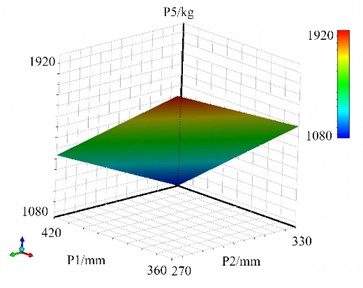
a) The response surface of P1 and P2 for P5
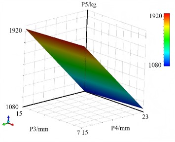
b) The response surface of P3 and P4 for P5
The response surface model between the stress peak and the design variables is shown in Fig. 13. Stress calculation relies on material mechanics, elasticity mechanics or finite element theory, and the relationship between stress and design variables is often derived through complex mechanical formulas. Due to the high-order power relationship between the moment of inertia of the cross-section and the cross-sectional dimensions, combined with the nonlinear finite element iterative solution, the response surface model becomes nonlinear. When subjected to bending loads, the flanges, being located far from the neutral axis, enable the steel to fully utilize its tensile and compressive strengths. This effectively transmits and distributes forces, allowing H-beams to excel in resisting bending deformation. Under lateral shear forces, the web efficiently transfers shear forces to the flanges, enabling them to jointly resist external forces. An increase in flange width significantly enhances the bending strength of H-beams, as the flanges primarily bear tensile and compressive stresses during bending. Wider flanges provide a larger section modulus, improving bending resistance. Appropriately increasing the thickness of the web can enhance its shear resistance, preventing shear failure caused by excessive shear forces. However, an overly thick web increases material usage, raising costs and potentially complicating self-weight control in structural design. Therefore, the optimal web thickness should be determined by balancing structural force requirements with economic considerations. Additionally, the cross-sectional height of H-beams plays a critical role in bending strength. Increasing the cross-sectional height substantially boosts the moment of inertia of the cross-section, thereby significantly enhancing the overall bending resistance.
Fig. 13The response surface models of P6
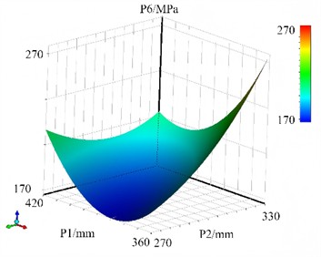
a) The response surface of P1 and P2 for P6
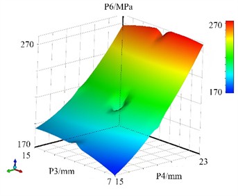
b) The response surface of P3 and P4 for P6
The response surface model between the first natural frequency and the design variables is shown in Fig. 14. The physical significance of the first natural frequency is the fundamental frequency of the overall vibration of the structure, and its magnitude is positively correlated with the overall stiffness of the structure. Therefore, the relationship with the design variables is centered on the overall stiffness change. The change of design variables will monotonically affect the overall stiffness, and thus the first natural frequency will show a monotonous trend. For example, increasing the section height of H steel will increase the section moment of inertia, enhance the overall stiffness, and the first natural frequency will monotonically increase (approximately in a quadratic relationship, as stiffness is related to the high power of dimensions). Nonlinearity is mainly caused by the high-order relationship between stiffness and variables (such as the cubic relationship between the moment of inertia and dimensions), but the overall nonlinearity is weaker than the response surface of the stress peak. From the perspective of structural mechanics, an increase in flange width enhances the moment of inertia of the cross-section, thereby improving the flexural rigidity of the structure. According to modal analysis theory, increased structural stiffness leads to a higher natural frequency. Simulation results indicate that as flange width increases gradually, the modal frequencies of all orders of the chassis frame exhibit an upward trend. In the first-order modal shape, reduced bending deformation reflects enhanced flexural capacity. Similarly, an increase in web height boosts the moment of inertia and flexural rigidity. However, excessive web height may compromise local stability. When evaluating the influence of web height on modal characteristics, both overall stiffness and local stability must be considered comprehensively. Within a certain range, increasing web height raises modal frequencies of the chassis frame. Beyond a critical value, however, local stability issues cause modal frequencies to decline. Additionally, higher-order modal shapes reveal intensified local vibrations in the web. Within a specific thickness range, stiffness enhancement dominates the increase in natural frequency. Finite element simulations altering flange and web thicknesses show that increased flange thickness slightly raises modal frequencies due to its significant contribution to flexural rigidity, which outweighs the effect of added mass. Conversely, changes in web thickness result in minimal modal frequency variations, as the web primarily resists shear forces and has limited influence on overall flexural rigidity.
Fig. 14The response surface models of P7
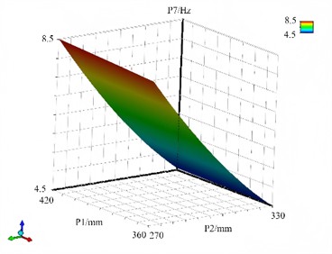
a) The response surface of P1 and P2 for P7
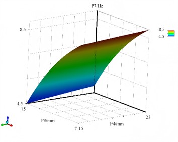
b) The response surface of P3 and P4 for P7
3.3. Analysis and discussion of optimization results
The flowchart of the optimization process for the chassis frame structure is shown in Fig. 15. If the response surface function is determined, an optimization mathematical model can be established. This model not only clarifies the criteria for selecting optimization variables but also provides a well-defined direction and theoretical foundation for subsequent optimization computations. As a widely adopted approximation modeling technique, the response surface method is primarily used to characterize the relationship between design variables and system responses, thereby simplifying complex engineering problems. The mathematical model derived from this method effectively captures the nonlinear and multivariate features of real-world problems in a more interpretable manner, facilitating further analytical exploration. When addressing multi-objective optimization problems, constructing a precise mathematical framework that reflects the problem's intrinsic characteristics becomes crucial. Multi-objective optimization typically involves multiple competing objectives – for instance, achieving both lightweight design and high structural strength in mechanical systems. In such scenarios, single-objective optimization strategies are often insufficient to meet comprehensive performance requirements. Therefore, a systematic mathematical formulation is required to reconcile trade-offs among conflicting objectives and identify the Pareto optimal solution set. These problems are conventionally transformed into formal mathematical expressions to enable rigorous analysis and comparative evaluation of performance improvements.
Fig. 15The response surface models of P7

Typically, an optimization mathematical model comprises three core components: objective functions, constraint conditions, and design variables. Objective functions represent the quantifiable performance metrics being optimized, such as minimizing structural mass, maximizing stiffness, or reducing energy consumption. Constraint conditions define the feasible region of the design variables, incorporating physical and engineering limitations such as dimensional bounds and material strength thresholds. Design variables, in turn, are the adjustable parameters that collectively determine the system’s final performance. Using this model, structural optimization can be formulated as a constrained multivariable nonlinear optimization problem. Such problems are generally associated with complex solution landscapes containing multiple local optima. Solving them requires efficient numerical algorithms and appropriate initial configurations. By iteratively adjusting and reconfiguring the design variables, it is possible to progressively approach the global optimal solution while satisfying all imposed constraints. Commonly employed optimization algorithms include gradient-based methods, genetic algorithms, and particle swarm optimization techniques, with the selection depending on the complexity and available computational resources. The constructed numerical optimization models are presented in Eq. (1) and Eq. (2). Eq. (1) defines the mathematical expression of the objective function, while Eq. (2) specifies the explicit or implicit constraint conditions that ensure the physical and engineering feasibility of the design. Together, these two equations form a complete mathematical optimization framework, serving as a robust basis for numerical computation and subsequent performance analysis. To maintain the structural integrity and stiffness of the chassis frame following lightweight design, the target parameters P6 and P7 are formulated as boundary conditions:
where is the maximum stress of the initial model, is the first-order natural frequency of the initial model.
Fig. 16Convergence curve of optimization solution
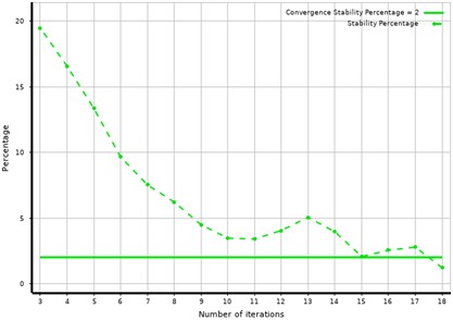
To address the challenges in solving mathematical models, this study adopted the Sequential Quadratic Programming (SQP) algorithm. During the implementation of this algorithm, the convergence curve of the iterative calculation is shown in Fig. 16, which clearly demonstrates its excellent convergence characteristics. As a mature optimization technique, SQP is widely recognized as one of the most effective methods for handling nonlinear constraint problems. The fundamental principle of SQP is to construct a quadratic programming sub-problem at each iteration to approximate the original nonlinear optimization problem, thereby gradually approaching the optimal solution. This method exhibits outstanding convergence, maintaining high computational accuracy and robust search performance even under complex constraint conditions. Moreover, it can accurately capture the behavior of the objective function within a local region with only a small number of data samples and express it in a compact algebraic form. These features make SQP particularly suitable for high-dimensional, nonlinear, and computationally intensive engineering optimization tasks. By locally approximating the objective function and constraint conditions, the algorithm significantly reduces computational complexity and enhances overall solution efficiency. In the context of multi-objective optimization problems, the SQP algorithm demonstrates remarkable flexibility. It allows for the reformulation of the model to independently identify the extrema of each objective function. This capability not only broadens the algorithm's applicability but also facilitates the identification of trade-offs among conflicting objectives, thereby accelerating convergence and improving the overall efficiency of the optimization process.
Through the search operation of target extremum, the relevant results of multi-objective optimization can be obtained, as shown in Table 6. From the data in the table, it can be seen that, without changing the inherent frequency of the structure and without increasing the peak stress, by using the surrogate model for in-depth analysis and optimization design, a significant effect of reducing the structural weight by 9.94 % was ultimately achieved. This optimization result not only demonstrates the efficiency and accuracy of the surrogate model in complex engineering problems, but also provides a scientific basis and feasible solution for the reasonable adjustment of quality redundancy in practical engineering applications. In fields such as aerospace and automotive manufacturing, this lightweight design is of great significance for improving overall performance, reducing energy consumption and saving material costs.
Table 6The result of multi-objective optimization
Parameters / Results | P1 / mm | P2 / mm | P3 / mm | P4 / mm | P5 / kg | P6 / MPa | P7 / Hz | Weight loss rate / % |
Initial value | 390 | 300 | 11 | 19 | 1422.85 | 264.13 | 5.69 | – |
Optimized value | 375.3 | 282.1 | 14.4 | 22.7 | 1281.42 | 264.06 | 5.69 | 9.94 % |
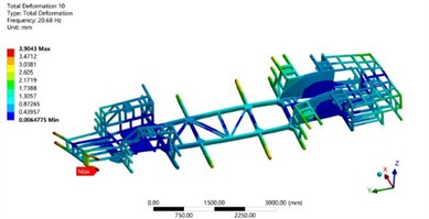
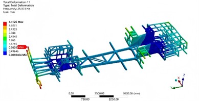
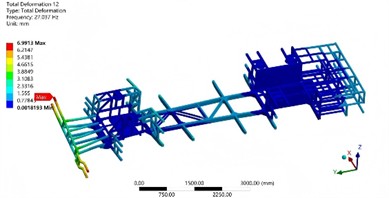
To further verify the reliability of the optimization results, the modal characteristics from the first to the sixth order before and after the optimization are compared as shown in Table 7. It can be seen that the natural frequencies from the second to the sixth order of the structure before and after optimization have no significant changes. The resonance position does not occur at the maximum load, which can ensure the safety and stability of the structure.
Table 7Comparison results of modal characteristics
Modal order | 1 | 2 | 3 |
Natural frequency of initial structure / Hz | 5.69 | 7.32 | 16.87 |
Natural frequency of optimized structure / Hz | 5.69 | 7.91 | 17.20 |
Modal shapes of optimized structure | 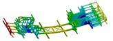 | 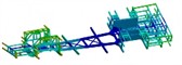 | 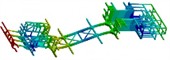 |
Modal order | 4 | 5 | 6 |
Natural frequency of initial structure / Hz | 24.34 | 25.53 | 31.07 |
Natural frequency of optimized structure / Hz | 24.07 | 26.64 | 30.97 |
Modal shapes of optimized structure | 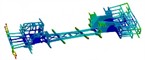 | 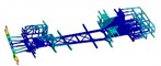 | 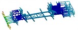 |
4. Conclusions
Based on the theory of multi-objective optimization, a structural optimization design scheme that comprehensively considers modal characteristics, strength requirements and lightweight requirements is proposed, aiming to enhance the overall vehicle performance while effectively reducing energy consumption. To achieve this goal, parametric finite element modeling of typical structures was implemented, and then modal and static characteristics were analyzed to obtain key performance indicators. Subsequently, the response surface method was used to construct an approximate model, and sample points were selected through experimental design methods to further fit the mathematical relationship between performance parameters and design variables. To ensure the reliability of the established model, significance tests and error analyses of the response surface function were also conducted to verify its accuracy in engineering applications. Through the solution and iterative analysis of the optimization model, a set of Pareto optimal solutions is ultimately obtained. The main conclusions are as follows:
1) The coupling parametric modeling method is an efficient modeling strategy that closely integrates multiple parameter variables with the model structure, significantly enhancing the efficiency and accuracy of finite element analysis. This approach enables the model to quickly generate calculation results that meet requirements during modal analysis and strength assessment. Such efficiency not only increases the degree of automation in the analysis process but also provides a solid foundation for subsequent multi-objective optimization design. Especially when dealing with complex engineering structures, coupling parametric modeling can achieve optimization goals such as lightweight, high strength, and high rigidity while meeting various performance indicators. Moreover, as this method supports flexible adjustment and iteration of parameters, it can effectively reduce the consumption of computing resources and shorten the simulation cycle during repeated calculations. This not only improves work efficiency but also ensures the acquisition of more accurate and stable discrete data sets.
2) The 40 sets of discrete data obtained through finite element analysis provide a solid foundation for establishing the functional relationship between design variables and optimization objectives. Based on these data, the response surface method can be used to construct an approximate model, thereby revealing the influence trends of each design variable on the optimization objective. Through error analysis of the fitting results, including calculating statistical indicators such as root mean square error and coefficient of determination, it is verified that the established response surface model not only has high prediction accuracy but also shows good stability, and can accurately reflect the behavioral characteristics of the actual structure. The study also introduced the Kriging interpolation method to construct a more accurate surrogate model. The Kriging model has unique advantages in handling nonlinear problems and can better capture the complex relationships between variables in the design space.
3) Based on the multi-objective optimization method, the scientific and reasonable adjustment of quality redundancy was effectively achieved. Without changing the strength and modal performance, the weight of the bus chassis frame was reduced by 9.94 %, achieving good economic and social benefits. The final analysis results show that this model demonstrates good adaptability and robustness in the lightweight design of vehicle frames, providing an effective tool for achieving a balance between structural performance and mass.
References
-
L. Rebhi, S. Khalfallah, A. Hamel, and A. Bouzar Essaidi, “Design optimization of a four-wheeled robot chassis frame based on artificial neural network,” Proceedings of the Institution of Mechanical Engineers, Part C: Journal of Mechanical Engineering Science, Vol. 239, No. 12, pp. 4756–4773, Feb. 2025, https://doi.org/10.1177/09544062251316755
-
C. L. Fu, Y. C. Bai, C. Lin, and W. W. Wang, “Design optimization of a newly developed aluminum-steel multi-material electric bus body structure,” Structural and Multidisciplinary Optimization, Vol. 60, No. 5, pp. 2177–2187, May 2019, https://doi.org/10.1007/s00158-019-02292-w
-
D. Wang, C. Xie, Y. Liu, W. Xu, and Q. Chen, “Multi-objective collaborative optimization for the lightweight design of an electric bus body frame,” Automotive Innovation, Vol. 3, No. 3, pp. 250–259, Jul. 2020, https://doi.org/10.1007/s42154-020-00105-1
-
A. Daşdemir, “A modal analysis of forced vibration of a piezoelectric plate with initial stress by the finite-element simulation,” Mechanics of Composite Materials, Vol. 58, No. 1, pp. 69–80, Mar. 2022, https://doi.org/10.1007/s11029-022-10012-7
-
S. M. Shohel, S. S. Gupta, and S. H. Riyad, “Weight optimization and finite element analysis of automobile leaf spring: A design construction referred to electric vehicle,” in IOP Conference Series: Materials Science and Engineering, Vol. 1259, No. 1, p. 012024, Oct. 2022, https://doi.org/10.1088/1757-899x/1259/1/012024
-
R. Talebitooti, H. D. Gohari, and M. R. Zarastvand, “Multi objective optimization of sound transmission across laminated composite cylindrical shell lined with porous core investigating Non-dominated Sorting Genetic Algorithm,” Aerospace Science and Technology, Vol. 69, No. 1, pp. 269–280, Oct. 2017, https://doi.org/10.1016/j.ast.2017.06.008
-
H. K. Celik, I. Akinci, N. Caglayan, and A. E. W. Rennie, “Structural strength analysis of a rotary drum mower in transportation position,” Applied Sciences, Vol. 13, No. 20, p. 11338, Oct. 2023, https://doi.org/10.3390/app132011338
-
S. Vulovic, M. Zivkovic, A. Pavlovic, R. Vujanac, and M. Topalovic, “Strength analysis of eight-wheel bogie of bucket wheel excavator,” Metals, Vol. 13, No. 3, p. 466, Feb. 2023, https://doi.org/10.3390/met13030466
-
K. J. Kim, “Light-weight design and fatigue characteristics of automotive knuckle by using finite element analysis,” Journal of Mechanical Science and Technology, Vol. 35, No. 7, pp. 2989–2995, Jun. 2021, https://doi.org/10.1007/s12206-021-0622-0
-
B. A. Nitalikar, D. R. Kulkarni, and Z. A. Patel, “Structural and finite element analysis of steering yoke of an automobile,” International Journal of Engineering and Management Research, Vol. 10, No. 5, pp. 168–175, 2020.
-
P. Purwanto, N. F. Qaidahiyani, M. S. Ikbal, and D. Djamaluddin, “Shear strength analysis of rock due to the effect of surface roughness based on laboratory testing and numerical modeling,” Materials Science Forum, Vol. 1091, No. 1, pp. 81–92, Jun. 2023, https://doi.org/10.4028/p-q863a9
-
J. Wang, C. Xu, Y. Xu, X. Qi, Z. Liu, and H. Tang, “Vibration analysis and parameter optimization of the longitudinal axial flow threshing cylinder,” Symmetry, Vol. 13, No. 4, p. 571, Mar. 2021, https://doi.org/10.3390/sym13040571
-
D. Perfetto, C. Pezzella, V. Fierro, N. Rezazadeh, A. Polverino, and G. Lamanna, “FE modelling techniques for the simulation of guided waves in plates with variable thickness,” Procedia Structural Integrity, Vol. 52, No. 1, pp. 418–423, Jan. 2024, https://doi.org/10.1016/j.prostr.2023.12.042
-
R. Talebitooti, M. Zarastvand, and H. Darvishgohari, “Multi-objective optimization approach on diffuse sound transmission through poroelastic composite sandwich structure,” Journal of Sandwich Structures and Materials, Vol. 23, No. 4, pp. 1221–1252, Jun. 2019, https://doi.org/10.1177/1099636219854748
-
O. Jassinbekov, M. Isametova, and G. Kaldan, “Development of a technique for computer simulation of the stress state of the drive drum shell of a belt conveyor to optimize its design parameters,” Eastern-European Journal of Enterprise Technologies, Vol. 2, No. 7 (110), pp. 31–39, Apr. 2021, https://doi.org/10.15587/1729-4061.2021.229213
-
H. D. Chalak, A. M. Zenkour, and A. Garg, “Free vibration and modal stress analysis of FG-CNTRC beams under hygrothermal conditions using zigzag theory,” Mechanics Based Design of Structures and Machines, Vol. 51, No. 8, pp. 4709–4730, Aug. 2023, https://doi.org/10.1080/15397734.2021.1977659
About this article

The paper is supported by provincial scientific research projects (62874155).
The datasets generated during and/or analyzed during the current study are available from the corresponding author on reasonable request.
The authors declare that they have no conflict of interest.
