Obtaining shear wave input for 1d site response analysis: a frequency adjustment method based on strong motion records – part i: formulation and theoretical validation

Wang, Yiping; Dong, Yinfeng; Wang, Yilin; Xie, Yiming; Cao, Fuchao

doi:10.21595/vp.2025.25272

Vibroengineering Procedia

Browse Procedia

Published: December 22, 2025

Check for updates

Obtaining shear wave input for 1d site response analysis: a frequency adjustment method based on strong motion records – part i: formulation and theoretical validation

Yiping Wang¹

Yinfeng Dong²

Yilin Wang³

Yiming Xie⁴

Fuchao Cao⁵

^{1, 2, 3, 4, 5}Key Laboratory of New Technology for Construction of Cities in Mountain Area, Chongqing University, Chongqing, China

^{1, 2, 3, 4, 5}School of Civil Engineering, Chongqing University, Chongqing, China

Corresponding Author:

Yiping Wang

Cite the article Download PDF

Downloads 16

Abstract

Significant discrepancies exist between strong motion records and the actual incident wave field across frequency bands, impacting wave propagation analysis accuracy. This paper proposes a frequency-domain adjustment method (AWIM) to derive realistic incident wave fields from recorded motions. The method constructs site-specific frequency adjustment curves by analyzing the steady-state response of soil layers to harmonic excitations using wave propagation theory and recursive calculations of reflection/transmission across layers. Results reveal that soft soil sites exhibit strong frequency-dependent effects: low-frequency waves undergo significant amplification (nearly twice the incident wave amplitude), while high-frequency waves show complex interactions – distinct bands experience notable amplification or attenuation.

Obtaining shear wave input for 1d site response analysis: a frequency adjustment method based on strong motion records – part i: formulation and theoretical validation

Highlights

Proposes a novel frequency-domain adjustment method (AWIM) to derive realistic incident wave fields from recorded strong motion data, addressing the discrepancy between total wave fields and ideal incident waves in 1D site response analysis.
Reveals significant frequency-dependent amplification in soft soil sites, with low-frequency waves amplified nearly twofold, while high-frequency waves exhibit complex amplification and attenuation patterns across distinct bands.
Introduces an efficient recursive wave propagation algorithm that terminates calculations when wave amplitudes decay below 0.05% of their original value, balancing computational accuracy and efficiency in multi-layered soil systems.

1. Introduction

For one-dimensional seismic response analysis, the main approaches include the Vibration Input Method (VIM) based on structural dynamics theory [1], the Wave Input Method (WIM) grounded in wave propagation theory [2], and the Finite Element Method (FEM) that uses numerical discretization to solve wave motion equations [3]. Among these, the wave input method (WIM) is particularly effective for analyzing multi-layered soil media and complex seismic wave fields [4]. It treats seismic waves as disturbances propagating through soil layers and calculates their propagation and response using transfer matrices [5] or wave equations. However, a key challenge arises when using borehole or bedrock acceleration records as input for WIM. These records represent a total wave field, including both incident and reflected waves, rather than the idealized incident wave field required for accurate wave propagation analysis. This discrepancy, especially prominent in low-frequency displacement responses, significantly limits the accuracy of site response analysis using conventional WIM. To address this issue, we propose a frequency-domain adjustment method (AWIM) to derive realistic incident wave fields from recorded motions.

2. Incident wave adjustment method

2.1. One-dimensional wave propagation analysis

The assumptions based on this paper are: one-dimensional layered medium, SH wave, linear elasticity, top free surface, and semi infinite substrate. Some parameters of soil involved are shown in Table 1.

Fig. 1 illustrates the wave propagation path in a one-dimensional soil system. In this study, each soil layer is treated as a homogeneous medium, with its density, shear wave velocity, thickness, and single wave propagation time in the soil layer denoted as $ρ_{i}$ , $v_{s, i}$ , $h_{i}$ , and $τ_{i}$ $(i = 1,2, \dots, n)$ , respectively. As shown in Fig. 1(c), when a shear wave propagates from the $i$ th layer to the $(i + 1)$ th layer, its reflection coefficient is denoted as $β_{1, i}$ ; when propagating from the $i$ th layer to the $(i - 1)$ th layer, the reflection coefficient is denoted as $β_{2, i}$ . The relation between above coefficients is given by:

1

- β_{2, i + 1} = β_{1, i} = \frac{ρ_{i} v_{s, i} - ρ_{i + 1} v_{s, i + 1}}{ρ_{i} v_{s, i} + ρ_{i + 1} v_{s, i + 1}}, i = 1,2, \dots, n - 1 .

For the ground surface (the $n$ th layer), it is assumed to be a perfect reflector. And for the bottommost layer of soil (the 1st layer), it is assumed to have no reflection.

Table 1Soil parameters of numerical model

Density	Shear wave velocity	Thickness	Single wave propagation time in the soil layer	Reflection coefficient	Damping ratio	The first-order angular frequency
$ρ$	$v_{s}$	$h$	$τ$	$β$	$ξ$	$ω$

Fig. 1Schematic diagram of the wave propagation model in soil

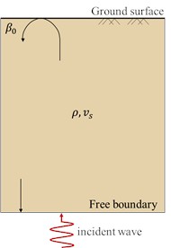
a) Wave propagation in single-layered media

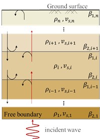
b) Wave propagation in multi-layered media

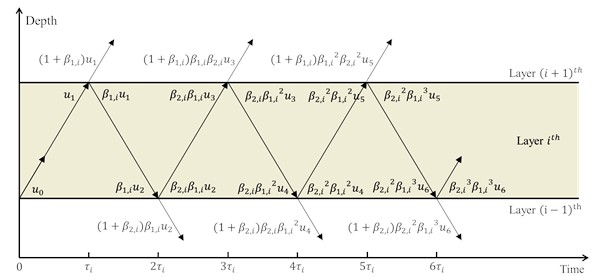
c) Wave propagation in the $i t h$ layer of soil

According to Fig. 1(c), the shear wave propagation from the bottom of the soil layer upward can be derived, including the wave responses at the top and bottom of each soil layer. The response at the top of the current layer and the transmitted shear wave into the upper layer can be expressed as:

2

p_{r u}^{-} (N τ_{i}) = p_{t u}^{-} (N τ_{i}) = (1 + β_{1, i}) \sum_{j = 1}^{N} \exp (- (2 j - 1) ξ_{i} ω τ_{i}) (β_{1, i} β_{2, i})^{j - 1} u_{2 j - 1},

where, $u_{2 j - 1}$ represents the shear wave in the soil layer that has shifted by $(2 j - 1) τ_{i}$ phases relative to the incident wave $u_{0}$ ; $N$ denotes the number of reflections of the shear wave in the soil layer, $ξ_{i}$ and $ω$ represent the damping ratio of the $i t h$ soil layer and the first-order angular frequency of the soil, respectively.

The reflected shear wave transmitted into the next soil layer $p_{t d}^{-}$ is:

3

p_{t d}^{-} (N τ_{i}) = (1 + β_{2, i}) β_{1, i} \sum_{j = 1}^{N} \exp (- 2 j ξ_{i} ω τ_{i}) (β_{1, i} β_{2, i})^{j - 1} u_{2 j} .

The response at the bottom of the current soil layer $p_{r d}^{-}$ is:

4

p_{r d}^{-} (N τ_{i}) = u_{0} + p_{t d}^{-} (N τ_{i}) .

Similarly, as the shear wave propagates downward from the top of the soil layer, the dynamic responses at both the top and bottom interfaces of each sublayer can be formulated as follows.

The response at the bottom of the current soil layer $p_{t u}^{+}$ and the transmitted shear wave into the next soil layer $p_{t d}^{+}$ are expressed as:

5

p_{t u}^{+} (N τ_{i}) = p_{t d}^{+} (N τ_{i}) = (1 + β_{2, i}) \sum_{j = 1}^{N} \exp (- (2 j - 1) ξ_{i} ω τ_{i}) (β_{1, i} β_{2, i})^{j - 1} u_{2 j - 1} .

The reflected shear wave transmitted into the previous soil layer $p_{t u}^{-}$ is:

6

p_{t u}^{-} (N τ_{i}) = (1 + β_{1, i}) β_{2, i} \sum_{j = 1}^{N} \exp (- 2 j ξ_{i} ω τ_{i}) (β_{1, i} β_{2, i})^{j - 1} u_{2 j} .

The response at the top of the current soil layer $p_{r u}^{+}$ is:

7

p_{r u}^{+} (N τ_{i}) = u_{0} + p_{t u}^{-} (N τ_{i}) .

To improve computational efficiency, this study sets the condition that wave propagation is terminated when the amplitude decays to less than 0.05 % of its original value due to damping. This threshold is expressed as $(β_{1, i} β_{2, i})^{N} \geq$ 0.05 %. Based on this threshold, the number of reflections $N$ of the shear wave in the $i t h$ soil layer is $N \geq \frac{\lg 0 . 05 %}{\lg (β_{1, i} β_{2, i})} \approx \frac{- 3.3}{\lg (β_{1, i} β_{2, i})}$ . By using above equations, the propagation of shear waves in the soil and the responses of each soil layer can be calculated using a recursive method.

2.2. Model validation

To assess the accuracy of the proposed model, a 500-meter soil column was extracted from a semi-infinite space and discretized into 1-meter elements. The soil properties were defined as a density of 2200 kg/m³ and a shear wave velocity of 200 m/s. A unit pulse shear displacement wave was introduced vertically upward at the base of the column, as shown in Fig. 2(a). Based on one-dimensional wave propagation theory, the shear wave reaches the midpoint of the column at 1.25 seconds (250/200 = 1.25), arrives at the top at 2.5 seconds (500/200 = 2.5), and is amplified by a factor of two due to the free surface at the top. The wave then reflects off the top surface and propagates downward, reaching the midpoint again at 3.75 seconds (750/200 = 3.75) and the base at 5 seconds (1000/200 = 5). After 7.0 seconds (1000/200+2 = 7.0), the shear wave completely exits the base and propagates to infinity. Following this, the displacement of each part of the model is calculated to be zero. The horizontal displacement response solutions at the bottom, middle, and top of the model are illustrated in Figs. 2(b) and 2(c) for damping coefficients of 0 and 400 kg/m³/s, respectively.

Fig. 2Model validation case

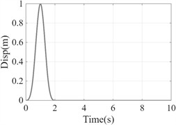
a) Incident wave

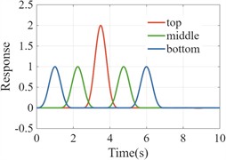
b) Undamped soil column response

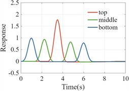
c) Damping soil column reaction

2.3. Incident wave adjustment method

For single-layer or multi-layer soils, when the frequency of the incident wave satisfies a specific multiple (or ratio) relationship with the natural frequency of the soil, the phase difference between the reflected and incident waves can cause amplification or attenuation of the wave field amplitude. Therefore, by analyzing the response of the site to harmonic excitations of different frequency, a specific frequency adjustment coefficient for the site can be obtained.

To determine the frequency adjustment coefficient of the soil, assume the soil layer thickness is $h$ , the shear wave velocity is $v_{s}$ , the density is $ρ$ , and the damping ratio is $ξ$ . A set of sine waves with different frequencies (amplitude set to 1) is input at the bottom of the soil layer. Based on wave theory and using the method described in above Section 2.1, the response at the bottom of the soil layer to the harmonic excitations of different frequency is calculated. The specific steps are as follows

(1) Determine the reflection and transmission coefficients $β$ . The reflection coefficient at the top of the soil is defined $β =$ 1, indicating total reflection.

(2) Time delay and propagation process. The time delay $τ$ for the seismic wave propagation through the soil layer is determined by the layer thickness $h$ and the shear wave velocity $v_{s}$ , i.e., $τ = h / v_{s}$ . The time delay determines the duration for both the reflected and transmitted waves to propagate through the soil layer, which in turn affects the frequency response characteristics.

(3) Input sine waves with different frequency. To study the response of a single-layer soil, a set of sine waves with different frequencies is chosen as the input wave. The expression for the input wave is given by:

8

x_{i n} (t) = \sin (2 π f_{i} t), t \in [0, T],

where $f_{i}$ is the frequency of the input wave, and $T$ is the total duration of the wave. After analyzing a large number of examples, it is recommended that the total duration $T$ should be at least ten sine wave periods to ensure the calculation accuracy. And to prevent the propagation time of high-frequency sine waves from being too short, we will increase the total duration by two seconds. In summary, $T$ should satisfy as $T \geq \frac{(2 + 10 t_{p} f_{i})}{f_{i}}$ , where 2 represents two seconds of increase, and 10 $t_{p} f_{i}$ represents ten sine wave periods. The number of time steps $n$ should meet the requirement that each sine wave is divided into $a$ or more parts:

9

n \geq \frac{a (2 + 10 t_{p} f_{i})}{f_{i} τ_{m i n}},

where $t_{p}$ is one-quarter of the inherent period of the soil, which can be simplified as $t_{p} = \sum_{i = 1}^{n} \frac{h_{i}}{v_{s, i}}$ , $τ_{m i n}$ is the minimum propagation time of soil wave for each layer, and $a$ is the number of time steps in one cycle of the sine wave. In the equation, $n$ is dimensionless, and the algorithm is more stable when $a \geq 20$ .

(4) Frequency adjustment coefficient. After the input wave propagates through the soil layers, it undergoes multiple reflections and transmissions, and its energy gradually reaches a steady state. By numerical simulation, the wave response at the bottom of the soil is calculated for different frequency sine wave inputs, and the steady-state amplitude of the signal is extracted, defined as the frequency domain amplification coefficient $ζ (f)$ :

10

ζ (f) = \frac{|x_{r e}|}{|x_{i n}|},

where $|x_{i n}|$ represents the amplitude of the input sine wave, and $|x_{r e}|$ denotes the amplitude of the envelope of the steady-state signal which includes the incident wave. To obtain the steady-state response, the envelope of the signal is extracted using the Hilbert transform (HT). The result of the Hilbert transform is given by $E n v (t) = |x (t) + i * Η (x (t))|$ .

(5) Adjust the strong motion records. The strong motion records are adjusted in the frequency domain based on the frequency domain amplification coefficient curve. First, motion records are subjected to a Fourier Transform (FT). Then, the amplitudes of different frequency bands are adjusted according to the frequency adjustment coefficient curve:

11

{\tilde{A}}_{a d j} (f) = \frac{{\tilde{A}}_{r e c} (f)}{ζ (f)},

where ${\tilde{A}}_{r e c} (f)$ represents the frequency-domain amplitude of the original seismic record, and $ζ (f)$ is the frequency adjustment coefficient mentioned above.

Finally, the adjusted frequency-domain amplitude is restored to the time-domain signal through the inverse Fourier transform (IFT), resulting in the adjusted incident wave field.

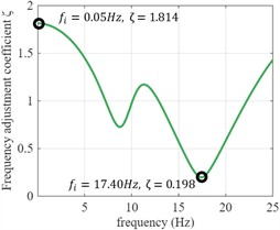
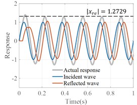
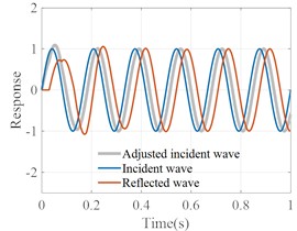
To better explain this method, a single-layer soil body is analyzed in this section, with parameters $h =$ 20 m, $v_{s} =$ 500 m/s, $ρ =$ 1914 kg/m³, $ξ =$ 0.0866. The whole adjustment process is shown in Fig. 3. Firstly, the response of the soil bottom under different frequency sine wave input is calculated, and the gray curve represents the bottom response in the response results. The blue and orange curves represent the sine wave input from the bottom and the reflected wave transmitted to the bottom, respectively. After the response reaches the steady state, obtain the adjustment coefficient $ξ$ corresponding to different sine wave frequencies, such as $f_{i} =$ 1 Hz, $ζ$ (2.5 Hz) = 1.705. By dividing the amplitude of each frequency band of the recorded seismic wave by the adjustment coefficient of the corresponding frequency band, the approximate incident wave can be obtained. In the lower right corner of Fig. 3, the whole adjustment process is shown.

The process of obtaining the frequency coefficient curve for the multi-layer soil model is similar to that of the single-layer soil model. By inputting sine waves of different frequencies as the initial signal and recursively calculating the reflected and transmitted waves at each layer using wave theory, the response at the bottom of the soil is obtained. For instance, consider a two-layer soil system, as shown in Fig. 4(a). Using an incident sine wave with a frequency of $f_{i} =$ 6 Hz as an example, the calculation and adjustment process is depicted in Fig. 4(c) and Fig. 4(d). After adjusting the sine wave in the frequency range 0 to 25 Hz, the frequency adjustment coefficient $ζ$ for the range 0 to 25 Hz can be obtained, as shown in Fig. 4(b). For a clearer explanation, we have presented a flowchart of the entire adjustment process, as shown in Fig. 5.

For different reflection truncation tolerances and different damping, the amplification factor curve will be different. Fig. 5 shows the influence of different reflection truncation tolerances and different multiples relative to the original damping on the adjustment coefficient by taking the multi-layer soil model in the above article as an example.

Fig. 3AWIM step

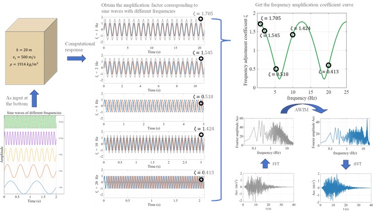
Fig. 4Multi-layer soil frequency adjustment coefficient and adjustment process

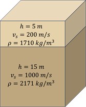
a) Multi-layer soil model

b) Frequency adjustment coefficient $ζ$

c) Pre-adjustment wave field ( $f_{i} =$ 6 Hz)

d) Post-adjustment wave field ( $f_{i} =$ 6 Hz)

Fig. 5The influence of different reflection truncation tolerances and different multiples relative to the original damping on the adjustment coefficient

The influence of different reflection truncation tolerances and different multiples relative to the original damping on the adjustment coefficient

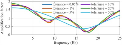
a) Different reflection truncation tolerances

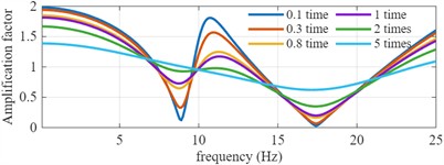
b) Different multiples damping

3. Conclusions

A frequency-domain adjusted wave input method (AWIM) to bridge the gap between recorded strong-motion records (total wave field) and the incident wave field required for one-dimensional site response analysis was proposed. By employing wave propagation theory and recursive layer calculations, site-specific frequency adjustment coefficients $ζ$ are derived to effectively link the incident wave field with the recorded strong-motion data. The advantage of this method is that the incident wave can be obtained without including the reflected part. The results show that both single-layer and multi-layer sites exhibit significant amplification effects on low-frequency incident waves, with amplification factors close to 2. For other frequency bands, the soil shows complex amplification and attenuation effects. In single-layer soil, these effects display a clear periodic pattern related to the shear wave velocity of the soil. However, in multi-layer soil, such periodicity is less evident.

References

Y.-B. Wang, X.-S. Huang, and C. Li, “The truncation effect of soil slope acceleration responses,” Soil Dynamics and Earthquake Engineering, Vol. 190, p. 109099, Mar. 2025, https://doi.org/10.1016/j.soildyn.2024.109099

Publisher
K. Mahmood, Z.-U.- Rehman, K. Farooq, and S. A. Memon, “One dimensional equivalent linear ground response analysis – A case study of collapsed Margalla Tower in Islamabad during 2005 Muzaffarabad Earthquake,” Journal of Applied Geophysics, Vol. 130, pp. 110–117, Jul. 2016, https://doi.org/10.1016/j.jappgeo.2016.04.015

Publisher
M. Koolivand, R. R. Ardakani, A. Mahdavian, and H. Saffari, “Simulation of the 2016 Kumamoto earthquakes using the finite element method with concentrated friction,” KSCE Journal of Civil Engineering, Vol. 27, No. 9, pp. 3824–3835, Sep. 2023, https://doi.org/10.1007/s12205-023-0031-2

Publisher
K. Koketsu, B. L. N. Kennett, and H. Takenaka, “2-D reflectivity method and synthetic seismograms for irregularly layered structures-II. Invariant embedding approach,” Geophysical Journal International, Vol. 105, No. 1, pp. 119–130, Apr. 1991, https://doi.org/10.1111/j.1365-246x.1991.tb03448.x

Publisher
Z. Shan, L. Jing, L. Zhang, Z. Xie, and D. Ling, “Transient wave propagation in a multi‐layered soil with a fluid surface layer: 1D analytical/semi‐analytical solutions,” International Journal for Numerical and Analytical Methods in Geomechanics, Vol. 45, No. 13, pp. 2001–2015, Jun. 2021, https://doi.org/10.1002/nag.3253

Publisher

About this article

Received

August 13, 2025

Accepted

November 10, 2025

Published

December 22, 2025

SUBJECTS

Seismic engineering and applications

DOI

https://doi.org/10.21595/vp.2025.25272

Keywords

wave propagation

seismic wavefield

site response

strong motion records

incident wave

Acknowledgements

The authors have not disclosed any funding.

Data Availability

The datasets generated during and/or analyzed during the current study are available from the corresponding author on reasonable request.

Conflict of interest

The authors declare that they have no conflict of interest.

This is an open access article distributed under the Creative Commons Attribution License, which permits unrestricted use, distribution, and reproduction in any medium, provided the original work is properly cited.

Previous article in issue Previous Next article in issue Next

Research article

2025 12 22

Obtaining shear wave input for 1D site response analysis: a frequency adjustment method based on strong motion records – part II: application to sites and the 2011 Tohoku earthquake

Yiping Wang, Yinfeng Dong, Yiming Xie, Fuchao Cao, Yilin Wang

Research article

2023 11 27

Characteristic period of response spectrum for surface and borehole ground motions

Qingshuang Su, Yinfeng Dong, Feiyu Guo, Xingyu Zhang

Research article

2023 10 20

Prediction of liquefaction time based on time-frequency distribution of seismic records

Hua Lu, Yanxin Yang, Xudong Zhan, Ziyun Lin

Y. Wang, Y. Dong, Y. Wang, Y. Xie, and F. Cao, “Obtaining shear wave input for 1d site response analysis: a frequency adjustment method based on strong motion records – part i: formulation and theoretical validation,” Vibroengineering Procedia, Vol. 60, pp. 97–103, Dec. 2025, https://doi.org/10.21595/vp.2025.25272

Copy Extrica

Copied to clipboard!

TY  - JOUR
DO  - 10.21595/vp.2025.25272
UR  - https://doi.org/10.21595/vp.2025.25272
TI  - Obtaining shear wave input for 1d site response analysis: a frequency adjustment method based on strong motion records – part i: formulation and theoretical validation
T2  - Vibroengineering Procedia
AU  - Wang, Yiping
AU  - Dong, Yinfeng
AU  - Wang, Yilin
AU  - Xie, Yiming
AU  - Cao, Fuchao
PY  - 2025
DA  - 2025/12/22
PB  - Extrica
SP  - 97-103
VL  - 60
SN  - 2345-0533
SN  - 2538-8479
ER  - 

Copy Ris

Copied to clipboard!

 @article{Wang_2025, title={Obtaining shear wave input for 1d site response analysis: a frequency adjustment method based on strong motion records – part i: formulation and theoretical validation}, volume={60}, ISSN={2538-8479}, url={https://doi.org/10.21595/vp.2025.25272}, DOI={10.21595/vp.2025.25272}, journal={Vibroengineering Procedia}, publisher={JVE International Ltd.}, author={Wang, Yiping and Dong, Yinfeng and Wang, Yilin and Xie, Yiming and Cao, Fuchao}, year={2025}, month=dec, pages={97–103} }

Copy Bibtex

Copied to clipboard!

[1]Y. Wang, Y. Dong, Y. Wang, Y. Xie, and F. Cao, “Obtaining shear wave input for 1d site response analysis: a frequency adjustment method based on strong motion records – part i: formulation and theoretical validation,” Vibroengineering Procedia, vol. 60, pp. 97–103, Dec. 2025, doi: 10.21595/vp.2025.25272.

Copy IEEE

Copied to clipboard!

Wang, Yiping, Yinfeng Dong, Yilin Wang, Yiming Xie, and Fuchao Cao. “Obtaining Shear Wave Input for 1d Site Response Analysis: A Frequency Adjustment Method Based on Strong Motion Records – Part i: Formulation and Theoretical Validation.” Vibroengineering Procedia 60 (December 22, 2025): 97–103. https://doi.org/10.21595/vp.2025.25272.

Copy Chicago

Copied to clipboard!

Obtaining shear wave input for 1d site response analysis: a frequency adjustment method based on strong motion records – part i: formulation and theoretical validation

Abstract

Highlights

1. Introduction

2. Incident wave adjustment method

2.1. One-dimensional wave propagation analysis

2.2. Model validation

2.3. Incident wave adjustment method

3. Conclusions

References

About this article

Related Articles