Abstract
Cross-domain fault diagnosis for rolling bearings under unseen working conditions is a challenging yet essential task, as the distribution bias significantly degrades the performance of data-driven methods. Causality-inspired domain generalization aims to address this challenge, with existing methods primarily focusing on alignment- or gradient-based operations from an entire signal perspective, which, however, overlooks the risk that biased alignments may induce spurious correlations and misguide learning. To this end, we reformulate the problem from a more physical and fine-grained perspective by treating fault-irrelevant frequency bands as confounders and aiming at localizing causal frequency bands encoded with robust and interpretable fault-related features to explicitly extract causal features. We propose a frequency band-aware method with a cyclostationarity-enhanced representation. Specifically, we first introduce a representation based on spectral correlation density (SCD) for wavelet packet-decomposed frequency bands. Then, treating cycle frequencies as channels, an adaptive feature extractor is designed based on a mixture-of-experts (MoE) block with a multi-view router, which integrates the views of spectrum, frequency band, and entire sample, to adaptively extract features across samples. In addition, prior knowledge guidance is introduced to enhance robust features. With cycle frequency-level features of frequency bands, a frequency band-aware attention module based on a tokenized Transformer, enhanced with an entropy-based sparsity regularization, is designed to model inter-band dependencies and localize fault-related frequency bands for diagnosis. Experiments are conducted on Case Western Reserve University (CWRU), Paderborn University (PU), and Harbin Institute of Technology (HIT) bearing datasets, and the proposed method shows effectiveness and interpretability across transfer tasks with different spans.
Highlights
- A frequency band-aware framework with cyclostationarity-enhanced representation is proposed to achieve interpretability with cycle-frequency and frequency-band as intermediate features and domain generalization with explicit extraction of causal features.
- A cycle-frequency-level feature extractor is designed based on mixture-of-experts with a multi-view router to activate sufficient features from spectral correlation density across domains, followed by a prior-knowledge-guided enhancer to emphasize robust fault-related ones.
- A frequency band-level localizer is constructed based on a tokenized Transformer with an entropy-based sparsity regularization to localize causal frequency bands for generalized fault diagnosis.
1. Introduction
Deep learning based rolling bearing fault diagnosis has gained widespread attention in recent years because of its strong capability of automatic feature extraction, which effectively circumvents physically modeling for sophisticated rotational mechanical systems and bias arising from manual feature extraction, e.g., CNN-based [1], autoencoder-based [2], deep belief network-based [3]. However, these models fail when applied to scenarios involving cross-working conditions. The underlying reasons stem from disparities in data distribution and limited availability and diversity of source data in the real-world industry. These two limitations directly contradict the fundamental premises of the traditional deep learning-based methods trained by the empirical risk minimization paradigm (ERM): the sufficiency of source data, and the independently and identically distributed (i.i.d.) condition of source and target data [4]. Recently, unsupervised domain adaptation has been studied to learn domain-invariant knowledge from the view of distribution alignment with unlabeled data of target domains, e.g., correlation alignment based on deep canonical correlation analysis [5]. However, in real-world industry, machines often operate in different working conditions, where collecting sufficient fault data and training condition-specific models is inefficient and costly. Therefore, it is necessary to further extend the deep learning-based fault diagnosis to achieve the generalization capability of rolling bearing fault diagnosis for cross-working condition scenarios under unseen ones.
Domain generalization is a branch within transfer learning, aiming at training a model from source domains with labels and directly generalizing to unseen target domains [6]. This theory particularly matches real-time fault diagnosis scenarios characterized by complex and frequent emergence of unseen working conditions. From the perspective of domain generalization, there are several paradigms proposed, including data augmentation [7-12], feature disentanglement [13-15], ensemble learning [16, 17], and meta-learning [18-20]. Recently, several studies [4, 21-28] have introduced causal mechanism as an advanced tool of feature disentanglement into cross-domain fault diagnosis with the assumption that data is made up of causal features and non-causal features, and the causal features is the key to achieving domain generalization. These existing causality-inspired fault diagnosis methods can be divided into two groups: feature separation [21, 22, 25, 26, 28-31], i.e., identifying and separating causal and non-causal features during model optimization, and feature purification [4, 27], i.e., obtaining causal features by removing non-causal features during model optimization. Feature separation introduces a hypothetical structural causal model based on data generation, with two unobservable variables as fault-related features and fault-irrelevant features respectively to block the spurious correlation between state label and working condition. The most popular approaches implementing feature separation are to design some specific loss functions to align or aggregate fault-related features and fault-irrelevant features, respectively. On the contrary, feature purification introduces a hypothetical structural causal model based on model inference. The most common approaches to implement feature suppression are to employ gradient-based operations, e.g., reversal and truncation.
However, existing causality-inspired data-driven methods have certain limitations: (1) limited transparent diagnostic procedure, (2) retention of spurious features, (3) limited capability for adaptive feature extraction.
– Limited transparent diagnostic procedure. Most existing methods derive from computer vision and time series processing, in which raw signals are directly fed into black-box feature extractors and classifiers to fit an abstract input-output relation. Such paradigms do not take the unique physical characteristics of mechanical monitoring signals, e.g. impulsiveness, cyclostationarity, into account during the design of the diagnosis model and lack the interpretability objectively. This leads to difficulty in further fault mechanism analysis and limited model improvability for future more complex cases. Therefore, we aim to find a more suitable input feature that is better suited for tracking the physical nature of faults and establishing a transparent diagnostic model.
– Retention of spurious features. Both feature alignment- and domain adversarial-based methods are fundamentally constrained by the diversity of source domains. The features obtained through alignment regularization or adversarial removal are inherently domain-dependent and biased with spurious features, i.e., the implicitly insignificant non-causal features absorbed as the common features of source domains. This problem can be attributed to the fact that domain-invariant features learned from biased data distributions are not necessarily causal and cannot adapt well to the unseen target domain, especially in cases with large distribution gaps [32]. [33] employed parallel multi-branch architectures to eliminate spurious features from multiple views. However, the architectural complexity arising from the large number of branches causes additional computational overhead, and the sensitivity of the type and number of branches limits the scenario adaptability.
Through literature review, we noticed that, in computer vision, some studies enhance domain generalization by identifying confounders from a more specialized view with physically interpretable and quantifiable variables, e.g., [32] treated scene context as confounders and used an attention invariance loss to capture image-level features of objects in the object detection task. Such physics-informed design clarifies the feature extraction targets and effectively suppresses confounder effects. This inspires us to rethink and identify confounders in cross-domain fault diagnosis.
We observe that the confounders in cross condition fault diagnosis primarily include variations caused by different rotation speed and load, e.g., different amplitude and different speed-dependent harmonics, environment noise, and sensor noise. To reflect these features from the complex structure of mechanical signals, the frequency domain is a well-known space with different mechanisms pertaining to different frequency bands, including fault-induced patterns, working condition-generated vibrations, and environmental noise [34]. Therefore, we formulate the problem from a more physical and fine-grained perspective by focusing on frequency bands, and treat frequency bands associated with environments and working conditions as confounders. Following this perspective, we aim to develop a module to localize the causal frequency bands associated with health state while filtering out environment-related frequency bands, to eliminate spurious features as much as possible, thereby boosting domain generalization and improving interpretability as well.
– Limited capability for adaptive feature extraction. Most existing models are conventional static models that apply the same processing to data from different domains. This is not effective enough because feature patterns are distinct across health states and working conditions. Even under identical working conditions, slight environmental differences may lead to inconsistent representations. To activate suitable features for different samples, [27] designed a dynamic convolution network with attention-guided weights from multiple views to adaptively extract features across different samples. But the complexity of multi-objective optimization within a single dynamic convolutional module introduces considerable complexity, making it difficult to optimize effectively. Therefore, it still lacks a suitable feature extractor for generalization across working conditions, which is the base for data-driven methods. Recently, [35] proved that a mixture-of-experts-based model trained with the ERM loss function is more robust to distribution shifts in target recognition than conventional models, e.g., ResNet50, trained with domain generalization strategies, as its architecture better aligns with invariant correlations. This motivates us to design a specific feature extractor based on a mixture-of-experts for cross-working-condition fault diagnosis to adaptively capture discriminative features from data of different domains.
Based on the above motivations, we propose a novel frequency band-aware method for cross-domain fault diagnosis with multi-source domains, incorporating cycle frequency-level adaptive feature extraction and frequency band-level causal localization. In general, our main contributions are summarized as follows:
1) A causal-interpretable framework for cross-domain fault diagnosis: A frequency band-aware framework with cyclostationarity-enhanced representation is proposed to achieve physical interpretability and domain generalization. This framework integrates two modules: (i) a cycle frequency-level module to capture the potential fault-related modulation patterns from spectral correlation density within each frequency band, (ii) a frequency band-level module to focus on causal frequency bands and suppress the spurious ones sensitive to domain shift.
2) A mixture-of-experts-based feature extractor with multi-view router: An adaptive cycle-frequency-level feature extractor is designed based on mixture-of-experts, equipped with a novel multi-view router considering the semantic dependency of cycle frequencies, enabling sufficient activation across samples from different domains. A prior-knowledge-guided enhancer is introduced to emphasize robust fault-related features.
3) A frequency band-aware localizer based on tokenized Transformer. A frequency band-aware localizer is built upon a tokenized Transformer with an entropy-based sparsity regularization, which extracts the frequency band-level patterns and focuses on causal ones for generalized fault diagnosis.
4) Excellent performance: The proposed model is validated on 3 datasets, covering cases of working-condition transfer with distribution gaps ranging from small to large. Remarkably, the proposed model achieves the highest overall average accuracy across all datasets, with particular improvement in large-span transfer tasks.
2. Related work
2.1. Multi-source domain generalization for fault diagnosis
Multi-source domain generalization is a rising perspective for addressing the generalization challenge in complex industrial environments of rotational mechanical systems by utilizing data from multiple source domains. Methods based on data augmentation aim to create data of pseudo domains assisted with source data. Typical methods include direct numerical operations, e.g., interpolation [36], and distribution-based combination, e.g., convex combination with Dirichlet-based Mixup [7]. Moreover, Wang et al. [12] proposed a collaborative domain-cycling framework with multiple feature domains and employed multiple metrics to filter high-quality data. However, the semantics evaluation of the augmented data is a challenging threshold for further investigation. Zheng et al. [37] proposed to use Local Fisher Discriminant Analysis (LFDA) to first obtain the optimal discriminant structure of each source domain, and then map the general mean subspace onto the Grassmann manifold as a general feature mapping transformation kernel for data from different domains. Explicit feature distribution alignment is a popular regularization view to constrain the model to learn general features from multiple source domains, e.g., MMD loss [38], triplet loss [39], and central loss [40]. To exploit the advantages of each source domains, Zhao et al. [16] trained domain-specific branches for each source domain with a similarity indicator branch to have a comprehensive evaluation. Gao et al. [19] proposed a meta-learning strategy to simulate the generalization scenario of industrial processes with meta-test sub-domains divided from source data to enhance learning general representation. Mu et al. [17] proposed a Theil index-based meta-learning network (TTIMN-GCS), where a task-orientated Theil index is designed to balance the inequality among meta-tasks to achieve a more generalized meta-optimization.
2.2. Causality-inspired domain generalization for fault diagnosis
Causality-inspired domain generalization methods can be divided into two groups: feature separation and feature purification. Feature separation methods typically construct a structural causal model (SCM) based on the data-generating process, followed by regularization based on do-calculus to extract causal variables [30, 26, 31]. Guo et al. [23] proposed a causal independence and sparse shift network (CIS2N), which samples intervention pairs with the same label from different domains and is trained with a causal independence loss based on independent causal mechanisms (ICM) and a sparse shifts loss based on sparse mechanism shifts (SMS). Jia et al. [29] found that solely taking causal factors into account leads to insufficient removal of the spurious correlation. To address this, they proposed a deep causal factorization network (DCFN), which adds a domain classification flow to extract non-causal factors. They [25] later extended it to a causal disentanglement domain generalization model (CDDG) by introducing generative modeling with a reconstruction loss. Another line of work is based on invariant risk minimization (IRM) and its variants, which treats data from each environment individually and learns an optimal classifier on top of a data representation matching all environments [41]. Mo et al. [42] proposed a sparsity-constrained invariant risk minimization method (SCIRM), which introduces differentiable sparsity regularizations to learn invariant classifiers across domains with sparse and effective features. The above works can be classified as class-conditioned methods, focusing on the invariant distribution of causal features conditioned on health state. However, Cheng et al. [22] noted that the distribution of causal features with the same label may shift due to the variation of bearings. Inspired by causal matching [43], they proposed a three-stage based domain generalization fault diagnosis method (LOODG) with an object-conditional domain invariant rule to align features of samples from different working conditions but similar bearing. In addition to regularization constraints-based approaches, Li et. al. [21] proposed Whitening-Net, which employs layer normalization (LN) to stabilize the distribution of individual sample and instance normalization (IN) to eliminate domain specific features. For models established upon feature purification, Wu et al. [4] proposed an adversarial-causal representation learning network (ACRLN) with spatial mask domain adversarial strategy using a gradient reversal layer and an auxiliary branch to remove domain specific features. Ma et al. [27] employed gradient truncation with the guidance of a binary mask created by domain discriminators to explicitly discard non-causal features at the layer and channel level. Besides, much research has employed masking mechanism guided by specific loss functions to purify causal features [44, 45]. Despite these advances, most existing domain generalization methods operate directly on the entire signal from an implicit perspective and rely heavily on neural network autonomy, which result in limited transparency and retention of spurious features.
3. Methodology
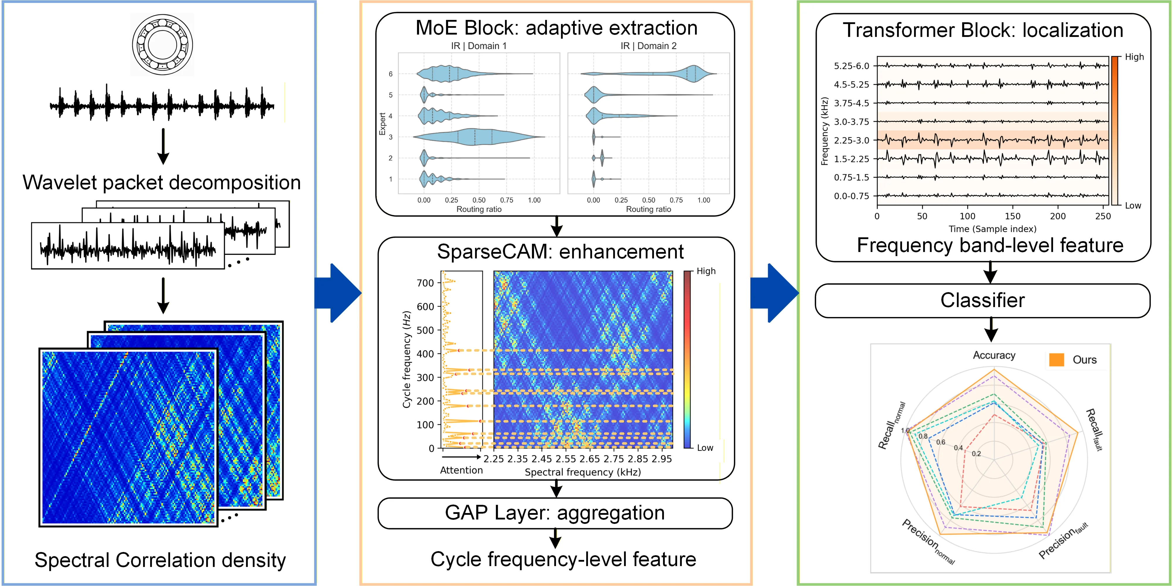
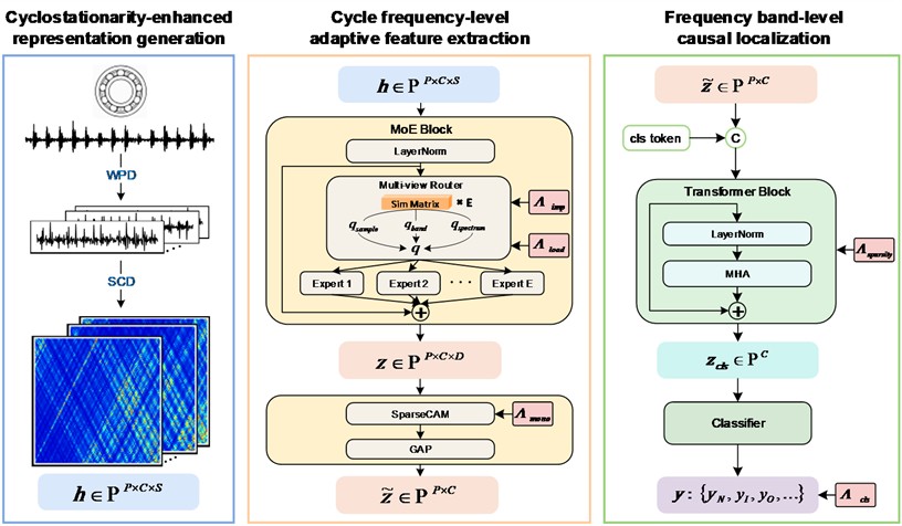
We propose a novel model for rolling bearing fault diagnosis under the multi-source domain generalization setting, as shown in Fig. 1, which consists of three stages: cyclostationarity-enhanced representation generation, cycle frequency-level adaptive feature extraction, and frequency band-level causal localization. First, we formulate the multi-source domain generalization problem for rolling bearing fault diagnosis in Section 3.1. In Section 3.2, we implement wavelet packet decomposition on the signal to divide it into patches corresponding to different frequency bands. Within each band, we calculate spectral correlation density to capture cyclostationarity as the input feature. In Section 3.3, we introduce a MoE block with a multi-view router to adaptively extract robust and suitable cycle frequency-level features. In Section 3.4, we introduce a frequency band-aware attention with sparsity regularization to localize causal frequency bands and suppress non-causal ones through quantifying the importance of frequency bands. Section 3.5 introduces the optimization objective and indicates the entire workflow.
Fig. 1Framework of the frequency band-aware multi-source domain generalization method for rolling bearing fault diagnosis
3.1. Problem definition
The domain generalization problem for rolling bearing fault diagnosis is set to recognize the health state of rolling bearing under unseen working conditions by acquiring generalizable knowledge from labeled data under multiple working conditions. In this context, let denotes source domains with each domain containing labeled data, where represents a vibration sample of length and is its corresponding label with health categories. Let denotes unseen domains with each domain containing unlabeled data of the -th unseen target domain. Due to the distribution shift under different working conditions, e.g. speed and load, the data distributions differ among source domains and between source and target domains, i.e., with , and , where , . The objective is to make full use of the source data to develop and optimize a method with good generalization to unseen domains.
3.2. Cyclostationarity-enhanced representation of frequency band
An effective representation is the core of a data-driven model. To establish a transparent diagnostic model, we choose to feed a representation based on cyclostationarity with spectral correlation density (SCD) which is a high-dimensional characteristic with the ability to reveal fault modulation frequencies.
– Frequency band decomposition with wavelet packets. First, to realize from the perspective of frequency bands, an input univariate time series is decomposed into patches corresponding to wavelet coefficients spanning from low-frequency to high-frequency bands, where is the length of wavelet coefficients. With a level wavelet packet decomposition, the input univariate time series is decomposed into patches, and patch captures the features of analyzed signal in the frequency range of . Each pair of wavelet coefficients at level and are calculated from through low-pass filter and high-pass filter respectively as:
The two filters are constructed with a scaling function and a selected primary wavelet function as:
where , which is the scaling function at a finer scale, is the inner product operator. Note that the two filters are mutually orthogonal with relationship of so that filtered signals through them are independent and represent low frequency band and high frequency band respectively.
– Cyclostationarity-enhanced representation. For the sake of effectiveness and interpretability, we choose spectral correlation density as the input feature, as it can effectively characterize the hidden periodic modulation mechanisms caused by different localized faults of rolling bearing through spectral correlation peaks, which provides a direct visualization of fault-induced modulation. As a classical feature of second order cyclostationarity, spectral correlation density is calculated based on the autocorrelation , where is the time shift. As the periodicity, it can be expanded into a Fourier series with cycle frequencies as:
where is defined as the cyclic autocorrelation function of cycle frequency , indicating modulation strength of cycle frequency . Then, it can be calculated by:
Then, the spectral correlation density can be calculated by the Fourier transform of the cyclic autocorrelation function with respect to the time shift as:
Based on Eq. (5), with the patches , we obtain the cyclostationarity-enhanced representation , where denotes the cycle frequency dimension, denotes the spectral frequency dimension. Each element of indicates the modulation strength of cycle frequency on spectral frequency .
3.3. Cycle frequency-level adaptive feature extraction
– Cycle frequency-level feature extraction via MoE with multi-view router. The adaptive feature extractor is designed based on a mixture-of-experts (MoE) block, which is a block of dynamically routed expert networks with each expert implemented by a feed-forward network (FFN). Specifically, input with the cyclostationarity-enhanced representation , the feed forward process is expressed as:
where denotes layer normalization used to stabilize the instance distribution, denotes the mixture-of-experts module which is given by:
where is the router of the gate calculating logits for assigning features to different experts, is an operation to only activate the top experts for each feature, specifically, it sets all other elements in the output vector as zero except for the elements with the largest logits, denotes an expert combined with a fully-connected neural network and a nonlinear activation function, and are hyperparameters representing the number of experts and the number of selected top experts respectively.
For the routing scheme, [35] shows that the cosine router achieves better performance than the linear router in domain generalization tasks because of its ability to mitigate the representation collapse issue. Specifically, the cosine router is calculated through cosine similarity among features and experts. Typically, the routing score for each token is computed as:
where represents the one-dimensional feature space for each expert, which assumes that each expert is responsible for a group of attributes with similar semantic. However, unlike visual tokens where each can represent specific attributes individually, e.g. ear, mouth, or leg, in this context where the tokens are cycle frequencies, the spectrum of single cycle frequency, i.e., the slice of the spectral correlation density function at a particular cycle frequency, can hardly exhibit clear semantic characteristics individually, e.g. fault, harmonic, or noise. The semantic of single cycle frequency commonly depends on both individual energy and the distribution structure of cycle frequencies [46, 47], which can be characterized by:
where denotes the modulation energy of , denotes the structural context including harmonic relationship , where represents the -th harmonic order, and sideband relationship , where the represents the rotational frequency. Moreover, to activate suitable and sufficient features for each cycle frequency of samples across different domains, we further evaluate the sample similarity to ensure that each expert focuses on cycle frequency with similar representation. To this end, we introduce a high-dimensional expert feature space as to evaluate comprehensively in routing. Then, for the high-dimensional input feature , the routing score is calculated from different dimensions, including spectral frequency (representing cycle frequency-level view), cycle frequency (representing frequency band-level view), and frequency band (representing sample-level view), which is expressed as:
where is a learnable matrix representing experts’ features, , and refers to the routing with features of spectral frequency, cycle frequency and frequency band respectively, denotes calculating the mean along dimension to get features of the rest dimension, is the projection function for input features mapping to a hypersphere, is a learnable parameter used to adjust the sharpness of the probability distribution to control the routing assignments. Through the above feature extraction, we obtain the cycle frequency-level feature .
– Auxiliary loss. To avoid the self-reinforcing imbalanced state that a gating network are prone to converge to, where a few experts are more frequently activated than others, followed [35], we optimize an importance loss , calculated with the square of coefficient of variation (CV) of total routing scores of all features to each expert, to encourage balanced routing scores across experts, and a load loss , calculated with the square of coefficient of variation of total assignment probabilities of all features to each expert, to encourage balanced assignment to ensure the sufficient usage of all experts:
where is the cumulative distribution function of a Gaussian distribution, is the -th largest routing score of each feature used as the threshold and only scores greater than it being assigned.
– Cycle frequency-level feature enhancement guided by prior knowledge. With the cycle frequency-level feature extracted by the MoE block, we employ a channel attention module (CAM) along the dimension of cycle frequency to highlight the fault-related cycle frequencies and enhance the corresponding features. The distribution of the fault-related cycle frequencies satisfies a sparsity property: the fault-related characteristic frequency and its harmonics are sparsely distributed at integer multiples of the fundamental frequency, while most other frequencies are irrelevant and redundant for diagnosis. However, the conventional Sigmoid layer produces smooth attention scores, which are insufficient for such sparsity. Inspired by [48], we redesign the channel attention with two branches: a squared ReLU-based branch that suppresses unrelated cycle frequencies with negative scores and propagates the most useful information flow forward, and a conventional Sigmoid-based branch that ensures sufficient information flow and keeps the model from falling into local optima during training. The process is expressed as:
where denotes the maximum operation, and are the parameter of fully connected layers.
Although the above design can effectively highlight informative cycle frequencies, we observe performance degradation when transferring across a large span from high-speed to low-speed conditions. Through analyzing the attention scores, we find out that fault impacts under high-speed conditions can trigger strong high-order harmonics, which provide a simple solution for the model. However, these high-order harmonics become weaker under low-speed conditions as the dominance of random vibrations over fault impulses [49] and lead the model to mistakenly recognize fault states as normal. To address this issue, we introduce a regularization term on scores produced by the channel attention module to encourage the model to pay more attention on low cycle frequencies while still retaining the ability to learn the discriminative feature from high cycle frequencies. The regularization term is calculated by:
where denotes the average score of the -th group cycle frequencies. This group-wise design is set to align with the discrete sparsity property of fault-related frequency distribution. The gradient of this regularization with respect to is derived as:
where . For each part, when , the corresponding item becomes to and to , thereby enforcing a monotonic decrease between adjacent group scores during backpropagation. When , the corresponding item will be truncated to control the scale of and prevent gradient explosion.
Then, a global average pooling layer (GAP) is used to aggregate each cycle frequency as:
In this way, we obtain the enhanced cycle frequency-level feature .
3.4. Frequency band-level causal localization
From the perspective of considering frequency bands associated with environments as confounders, a frequency band-aware module is proposed to localize fault-related frequency bands and suppress the influence of environment-related frequency bands.
– Localization with self-attention. To implement classification with the extracted features of frequency bands, inspired by prior work on modeling multiple sub-information in the classification of time series [50], we adopt a tokenized Transformer based on the self-attention mechanism of frequency bands. The tokenized Transformer tends to be popular in computer vision and time series, since it has been proven in [50] that it can reduce the complexity of developing a good classifier by explicitly modeling the correlation among input elements and lowering the class-conditioned entropy, which measures the uncertainty of features given that the class label is known. This means that employing a class token to aggregate features of causal frequency bands through modeling their correlations lowers the difficulty of classification compared to directly feeding raw features of frequency bands into a classifier. Additionally, the attention mechanism helps generate relation intensity graphs to visualize the importance of each frequency band. Here, we first employ a learnable class token to aggregate the features of causal frequency bands.
Specifically, we concatenate the class token with the features to yield a tokenized bag and aggregate fault-related information to update as:
where is the parameter of a fully connected layer used to fuse the output of multiple attention heads, denotes a self-attention head expressed as:
where , and are the parameters of the transformation layers. Nystrom attention [51] is used here to reduce the complexity of computation.
After the Transformer block, we only pass the class token to the classifier to make a prediction. To guide the learning of fault-related features and causal frequency band, the cross-entropy loss is used to perform classification with the prediction of classifier as:
where is the class label, is the batch size.
– Sparsity regularization for causal frequency bands. Beyond the tokenized Transformer, some spurious frequency bands may remain. Considering the difficulty in convergence and tuning of gradient-related methods, e.g., gradient reversal, and the obstacle of obtaining accurate domain labels, we purify causal frequency bands from another perspective, sparsity. Prior studies [52, 53] have proven that the health-related frequency bands are much fewer than those related to environments, and [54] has proven that causal features are much sparser than spurious ones. Moreover, some studies in causal representation learning have shown that applying sparsity regularization on the adjacency matrix of features helps prevent the model from overfitting and spurious solutions [55]. Motivated by these, we introduce an entropy-based sparsity regularization on the attention scores to encourage only a few frequency bands with significant values while the rest close to zero. Because, based on the definition of entropy [56], a lower entropy indicates a more concentrated probability distribution, which leads to a concentrated attention along frequency bands here. The sparsity regularization is expressed as:
where denotes the attention probability associated with the -th frequency band.
3.5. Training and inference
Beyond the above regularizations, the overall optimization objective is summarized as:
where , and are the balancing parameters.
The workflow of the proposed method is presented in Table 1.
4. Experiments
4.1. Dataset description
We study the performance of the proposed model with 3 datasets as follows, and their key attributes are summarized in Table 2, the test rigs are shown in Fig. 2.
Case Western Reserve University Bearing Dataset [57]. This is a vibration signal dataset that contains vibration signals collected by acceleration sensors from 6205-type ball bearings of 4 individual health states in different severities under 4 working conditions. The 4 health states include normal (N), inner race fault (IR), outer race fault (OR), and ball fault (B). These faults are single-point faults produced through electro-discharge machining with fault diameters of 7 mils, 14 mils, and 21 mils. The vibration signals are collected with a 12 kHz sampling frequency.
Paderborn University Bearing Dataset [58]. This is a vibration signal dataset collected by acceleration sensors from 6203-type ball bearings of 4 health states in different severities under 4 working conditions. We focus on 3 health states: normal (N), inner race fault (IR), and outer race fault (OR). These faults are single-point faults generated through life-accelerated degradation processes (e.g., pitting and indentations) with fault diameters ranging from less than 2 mm to more than 4.5 mm. The vibration signals are collected with a 64 kHz sampling frequency. In our experiments, to preserve enough revolutions for each sample, we downsample the data to 12 kHz.
Harbin Institute of Technology Bearing Dataset [59]. This is a vibration signal dataset that contains vibration signals collected by acceleration sensors from ball bearings of 3 individual health states on a real aeroengine under 25 working conditions. The 3 health states include normal (N), inner race fault (IR), and outer race fault (OR). These faults are produced through wire cutting with a fault depth of 0.5 mm and a fault length of 0.5 mm. The vibration signals are collected with a 25 kHz sampling frequency.
Table 1Workflow of the proposed rolling bearing fault diagnosis method
Algorithm: Frequency band-aware multi-source domain generalization method |
// Training Input: Source domain Model: Cyclostationarity-enhanced representation module , mixture-of-experts block , cycle frequency enhancer , band filter , classifier , and class token . Balancing parameters , , . 1 Initialize: model parameters , , , , 2 for training epoch do 3 for batch do 4 Sample one batch from 5 Decompose into wavelet packets 6 7 8 9 Add class token: 10 11 12 Calculate according to Eq. (19) 13 Calculate and according to Eq. (11) and (12) 14 Calculate according to Eq. (14) 15 Calculate according to Eq. (20) 16 Calculate according to Eq. (21) 17 Update , , , with back propagation 18 end 19 end Output: Trained parameters , , , , // Inference Input: Target domain Model: , with trained , with trained , with trained , classifier with trained , and trained class token . Output: Diagnosis results of |
Table 2Detailed configuration of experiment data
Dataset | Bearing | Case index | Speed (rpm) | Load | Health state |
CWRU | 6205 | C1 | 1797 | 0-HP | N, IR, OR, B |
C2 | 1772 | 1-HP | |||
C3 | 1750 | 2-HP | |||
C4 | 1730 | 3-HP | |||
PU | 6203 | P1 | 1500 | 1000-N | N, IR, OR |
P2 | 900 | 1000-N | |||
P3 | 1500 | 1000-N | |||
P4 | 1500 | 400-N | |||
HIT | 15 balls 30-mm 65-mm 7.5-mm | H1 | 1500-2500 | 0-N | N, IR, OR |
H2 | 3000-3700 | 0-N | |||
H3 | 3800-4100 | 0-N | |||
H4 | 4200-4500 | 0-N |
4.2. Implementation details
In our experiments, each sample’s vibration data is first resampled using angular resampling, following [60], to align signals such that each revolution contains an equal number of sampling points within each sample. Specifically, each sample consists of 2048 sampling points, corresponding to 4 revolutions with 512 points per revolution. The Haar wavelet is used as an example. For each sub-signal of frequency band, we set the number of cycle frequency as 128. For the MoE block, we set 6 experts, where each expert consists of 2 MLP layers (256 hidden neurons and a GELU activation) with a learnable similarity matrix of size . For each input feature, the multi-view router selects the TOP-1 expert index out of 6 and routes it to the corresponding one. The multi-head attention mechanism is configured with 8 heads.
Fig. 2Test rigs of each dataset
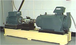
a) CWRU dataset
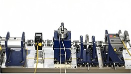
b) PU dataset
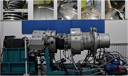
c) HIT dataset
In the training process, an AdamW optimizer is adopted with a weight decay of 3×10⁻⁴ and an initial learning rate of 1×10⁻⁴, which decays with a cosine annealing schedule. The balancing parameters and follow a cosine-based growth schedule from 0.01 to 1.0 and from 0.01 to 0.1, respectively, and is set to be a fixed value of 0.01. For , the cycle frequencies are divided into 16 groups, with each consists of 8 adjacent cycle frequencies. Training in the following experiments is performed over 300 iterations with a batch size of 128. All experiments are conducted with Pytorch in Python on an NVIDIA GeForce RTX 2080 Ti GPU.
4.3. Performance comparison experiments
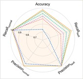
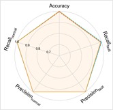
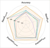
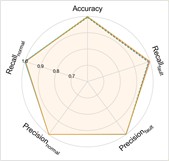
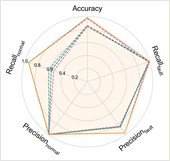
We first test our method in 3 cases with a gradually increasing level of difficulty. In these case studies, we compare our model with the recent representative baseline methods of multi-source domain generalization for bearing fault diagnosis: WhiteningNet [21], DGNIS [16], CDDG [25], ACRLN [4], CIMSDG [27]. In addition, we select an ensemble method using 19 traditional multi-domain features [61] as the basic baseline to evaluate the difficulty of tasks. To ensure the reliability and effectiveness of the experiment results, we conduct experiments for each method five times for each task. The diagnosis performance is indicated with five performance indicators, which are accuracy, fault recall, fault precision, normal recall, and normal precision, defined as:
– Case 1 (Cross-domain transfer on CWRU dataset): With 4 distinct working conditions, we establish 4 different cross-domain tasks. The data are balanced among 4 health states, with 300 samples for each health state in each source domain and 300 samples for each health state in each test domain.
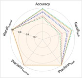
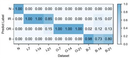
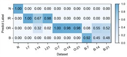
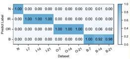
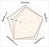
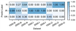
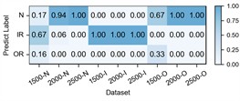
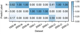
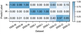
The experimental results of our method, along with the baseline methods, are presented in Table 3 and Fig. 3. Additionally, the comparison results of the detailed performance on each sub-dataset for C2+C3+C4→C1 are shown in Fig. 4. Our model achieves the highest overall average accuracy of 99.33 %. It can be observed that our model and the comparison methods all perform well with only a small performance gap among them. It is because the vibration data in the CWRU dataset has already been denoised and the distribution gap is small in this case, thus, the improvement from adaptive feature extraction with causal localization is not obvious as in the following cases.
Table 3Performance under different working conditions in Case 1
Model | Fault diagnostic average accuracy (%) | ||||
C2+C3+C4→C1 | C1+C3+C4→C2 | C1+C2+C4→C3 | C1+C2+C3→C4 | Average | |
Base | 94.39±0.06 | 99.31±0.05 | 97.91±0.00 | 90.75±0.05 | 95.59 |
WhiteningNet | 91.68±2.01 | 86.20±1.50 | 95.59±1.96 | 93.61±0.91 | 91.77 |
DGNIS | 83.34±2.09 | 95.39±0.50 | 92.84±3.16 | 96.66±1.25 | 92.06 |
CDDG | 97.72±2.61 | 97.12±1.61 | 99.82±0.13 | 92.54±0.46 | 96.80 |
ACRLN | 93.55±3.27 | 99.48±0.22 | 99.16±0.44 | 97.29±1.54 | 97.37 |
CIMSDG | 95.71±1.54 | 99.97±0.05 | 99.97±0.05 | 99.58±0.39 | 98.81 |
Ours | 98.68±0.93 | 99.62±0.34 | 99.90±0.15 | 99.12±0.26 | 99.33 |
Fig. 3Performance comprehensive comparison in Case 1
a) C2+C3+C4→C1
b) C1+C3+C4→C2
c) C1+C2+C4→C3
d) C1+C2+C3→C4

Fig. 4Detailed performance on each sub-dataset of case 1: C2+C3+C4→C1
a) WhiteningNet
b) DGNIS
c) CDDG

d) ACRLN
e) CIMSDG
f) Ours
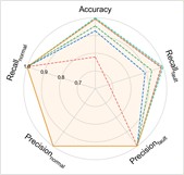
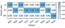
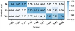
– Case 2 (Cross-domain transfer from real fault to real fault on PU dataset): With 4 distinct working conditions, we establish 4 different cross-domain tasks. The experimental protocol employs 9 sub-datasets, including 3 normal sub-datasets (K001, K002, K003), 3 inner race fault sub-datasets (KI14, KI16, KI17), and 3 outer race fault sub-datasets (KA04, KA15, KA16). The data are balanced among 3 health states, with 1200 samples for each health state in each source domain and 1200 samples for each health state in each test domain.
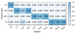
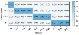
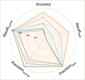
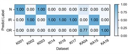
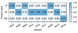
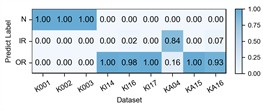
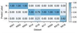
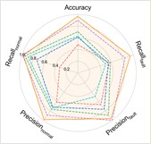
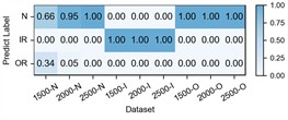
The experimental results of our method, along with the baseline methods, are presented in Table 4 and Fig. 5. Additionally, the comparison results of the detailed performance on each sub-dataset for P1+P3+P4→P2 are shown in Fig. 6. Our model achieves high accuracy among all cases and the highest overall average accuracy of 97.79 %. In the most challenging case (P1+P3+P4→P2), our model recognizes better in each sub-dataset and reaches a total accuracy of 94.25 % with a 21.84 % improvement over the best compared method. We also observe that our model has an average accuracy of 72 % on KA15, since the damage type of outer race fault in KA15 (indentations) is different from K04 and K16 (pitting). Although diagnosis under such difference is not the focus of this paper, our model can still handle it to a certain extent.
Table 4Performance under different working conditions in Case 2
Model | Fault diagnostic average accuracy (%) | ||||
P2+P3+P4→P1 | P1+P3+P4→P2 | P1+P2+P4→P3 | P1+P2+P3→P4 | Average | |
Base | 94.86±0.88 | 61.99±0.55 | 93.59±0.07 | 61.08±0.22 | 77.88 |
WhiteningNet | 99.61±0.15 | 62.78±4.29 | 99.57±0.16 | 83.01±1.32 | 86.24 |
DGNIS | 99.64±0.00 | 70.53±3.60 | 99.88±0.03 | 84.47±1.24 | 88.71 |
CDDG | 99.84±0.07 | 64.18±1.28 | 99.61±0.14 | 83.79±0.67 | 86.86 |
ACRLN | 99.88±0.07 | 56.56±2.28 | 99.83±0.19 | 92.87±1.10 | 87.29 |
CIMSDG | 100.00±0.00 | 72.41±1.39 | 100.00±0.00 | 88.32±1.42 | 90.18 |
Ours | 99.90±0.12 | 94.25±1.72 | 99.91±0.07 | 97.11±0.41 | 97.79 |
Fig. 5Performance comprehensive comparison in Case 2
a) P2+P3+P4→P1
b) P1+P3+P4→P2
c) P1+P2+P4→P3
d) P1+P2+P3→P4
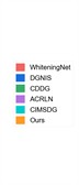
Fig. 6Detailed performance on each sub-dataset of case 2: P1+P3+P4→P2
a) WhiteningNet
b) DGNIS
c) CDDG
d) ACRLN
e) CIMSDG
f) Ours
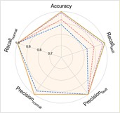
– Case 3 (Cross-domain transfer from artificial fault to artificial fault on HIT dataset): This case is designed to evaluate the transfer performance under large-span working conditions. We establish 4 different cross-domain tasks. The data are balanced among 3 health states, with 270 samples for each health state in each source domain and 270 samples for each health state in each test domain.
The experimental results of our model, along with the baseline methods, are presented in Table 5 and Fig. 7. Additionally, the comparison results of the detailed performance on each sub-dataset for H2+H3+H4→H1 are shown in Fig. 8. Our model achieves high accuracy among all cases and the highest overall average accuracy of 97.95 % among comparison methods. In the most challenging case (H2+H3+H4→H1), our model recognizes outer race fault under working condition of low speed (1500-O) and reaches a total accuracy of 96.79 % with a 6.91 % improvement over the best compared method. This demonstrates that, even in the case of large-span transferring from high-speed condition to low-speed condition, our model can handle the weak fault characteristics and maintain good performance.
Table 5Performance under different working conditions in Case 3
Model | Fault diagnostic average accuracy (%) | ||||
H2+H3+H4→H1 | H1+H3+H4→H2 | H1+H2+H4→H3 | H1+H2+H3→H4 | Average | |
Base | 66.79±0.20 | 81.73±0.40 | 92.92±0.25 | 83.91±0.11 | 81.34 |
WhiteningNet | 48.54±5.26 | 83.17±0.65 | 96.21±2.31 | 84.28±2.34 | 78.05 |
DGNIS | 61.16±3.17 | 83.29±1.23 | 97.24±0.68 | 85.88±1.96 | 81.89 |
CDDG | 70.64±0.94 | 82.63±1.36 | 97.45±0.15 | 85.84±1.53 | 84.14 |
ACRLN | 89.88±3.06 | 97.53±1.05 | 99.47±0.36 | 96.46±3.87 | 95.84 |
CIMSDG | 63.09±2.85 | 98.72±0.73 | 100.00±0.00 | 97.99±1.24 | 89.95 |
Ours | 96.79±0.97 | 97.12±0.42 | 99.84±0.23 | 98.03±0.27 | 97.95 |
Fig. 7Performance comprehensive comparison in Case 3
a) H2+H3+H4→H1
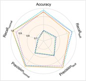
b) H1+H3+H4→H2
c) H1+H2+H4→H3
d) H1+H2+H3→H4

Fig. 8Detailed performance on each sub-dataset of case 3: H2+H3+H4→H1
a) WhiteningNet
b) DGNIS
c) CDDG
d) ACRLN
e) CIMSDG
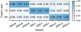
f) Ours
5. Analysis
In this section, we validate the improvements of the proposed method. For evaluation, we take the most challenging transfer scenarios from each of the three cases (C2+C3+C4→C1, P1+P3+P4→P2, and H2+H3+H4→H1) as examples, and conduct all ablation experiments for each method five times to ensure the effectiveness.
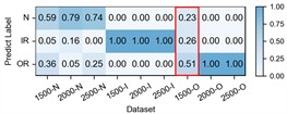
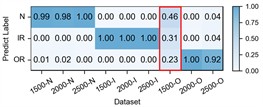
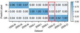
– Visualization of frequency band and cycle frequency. The frequency band-level decision-making mechanism and cycle frequency-level feature extraction make the proposed method interpretable. Leveraging these mechanisms, we obtain attention maps that highlight the model’s focus in diagnosis. The attention maps corresponding to the three health states (normal, inner race fault, outer race fault) in cases (C2+C3+C4→C1, P1+P3+P4→P2, and H2+H3+H4→H1) are visualized in Fig. 9. It can be observed that the proposed method effectively localizes the fault-related frequency band. At the cycle frequency level, the proposed model highlights the key cycle frequencies for fault states, while the attention for normal states is relatively uniform. These shows that the proposed method can purify fault-related features and reveal the fault modulation.
Fig. 9Exemplary attention maps of three health states (columns) in three cases (rows)
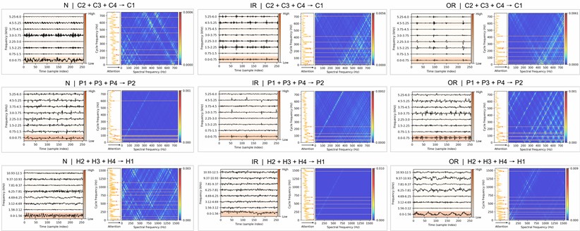
Table 6Physical features used for analyzing frequency band attention rankings
Index | Physical features | Expression |
1 | Mean of CSD | |
2 | Variance of CSD | |
3 | Max of CSD | |
4 | Skewness of CSD | |
5 | Kurtosis of CSD | |
6 | Energy of CSD | |
7 | Bandwidth of CSD | |
8 | Modulation index of CSD | |
9 | Spectral entropy of CSD | |
10 | Root mean square | |
11 | Variance | |
12 | Peak to peak value | |
13 | Kurtosis | |
14 | Crest factor | |
15 | Clearance factor | |
16 | Impulse factor | |
17 | Shape factor | |
18 | Skewness | |
19 | Shannon entropy |
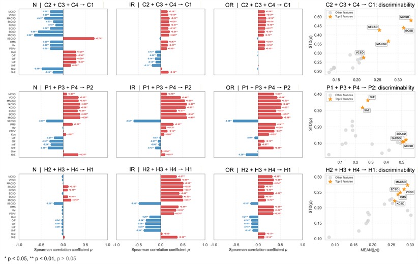
To further understand the features learned by the model, we make a correlation analysis between frequency band attention rankings and 19 actual physical features, as listed in Table 6, including 9 cyclic spectral features and 10 time domain features to identify those representative patterns learned by the model. From the results shown in Fig. 10, we see that: (1) for the case of C2+C3+C4→C1, AMICSD, BCSD, SECSD, MACSD are highly correlated with the frequency band attention rankings and high standard deviation across health states suggests that they may represent discriminative patterns captured by the model, (2) for the case of P1+P3+P4→P2, SECSD, AMICSD and SkCSD are highly correlated with the frequency band attention rankings and time domain features ShF and ShE are discriminative across health states, (3) for the case of H2+H3+H4→H1, MACSD, VCSD, ECSD, RMS and KCSD are highly correlated with the frequency band attention rankings and discriminative across health states.
Fig. 10The correlation analysis between frequency band attention rankings and actual physical features of three health states (columns) in three cases (rows). Left: Spearman correlation coefficients ρ between frequency band attention rankings and actual physical features. Right: feature scatter plots for each case, with the top 5 features ranked by MEANρ×STDρ highlighted with stars
– Ablation: Prior knowledge’s guidance in cycle frequency-level attention. The proposed prior-knowledge-guided channel attention module is used to reduce noisy representative features and redundant information while retaining the informative and relevant ones. Table 7 shows the ablation results that our designed module achieves the highest accuracy while the traditional one with Sigmoid obtains the lowest one. Fig. 11 illustrates the detailed performance comparison for the case H2+H3+H4→H1 and an example showing the different distributions of cycle frequency attention scores across the three methods. For the outer race fault under low-speed condition of 1500 rpm, our method achieves a remarkable improvement with an average accuracy of 86 % and a best-case performance of 97 %. In contrast, the Sigmoid-based approach shows unstable performance with an average accuracy of 51 %, while the Fusion-based approach almost fails to recognize the fault in this case with an average accuracy of 23 %. Furthermore, the proposed method also achieves more accurate and stable recognition for other states across other working conditions. From Fig. 11(f), it can be observed that our method guides the model to focus more on the low cycle frequency range with sparse attention, which helps keep the model from falling into a trivial solution when transferring from high-speed to low-speed conditions. These demonstrate that prior-knowledge-guided channel attention module makes the informative context be fully and correctly exploited while suppressing the redundant features, achieving a clear performance improvement.
Table 7Ablation of Prior knowledge’s guidance in cycle frequency-level attention
Prior knowledge’s guidance | Sigmoid | Fusion | Ours | |
Accuracy (%) | Case 1: C2+C3+C4→C1 | 97.24±2.49 | 98.12±2.22 | 98.68±1.14 |
Case 2: P1+P3+P4→P2 | 92.12±2.78 | 92.61±1.48 | 94.25±2.11 | |
Case 3: H2+H3+H4→H1 | 84.67±6.04 | 90.16±4.59 | 96.74±0.97 | |
Fig. 11Ablation of Prior knowledge's guidance in cycle frequency-level attention: The first row illustrates the detailed performance of three methods on each sub-dataset of case 3: H2+H3+H4→H1 with a) Sigmoid, b) Fusion, c) Ours. The second row provides an example of an outer race fault with d) raw vibration signal, e) the corresponding spectral correlation density of the first frequency band after decomposition, f) distributions of cycle frequency-level attention scores generated by three methods
a) Sigmoid
b) Fusion
c) Ours
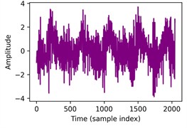
d) Raw vibration signal
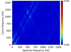
e) SCD of the first band
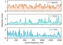
f) Attention scores
– Ablation: sparsity regularization on frequency band-level attention. Table 8 shows the results that the entropy-based sparsity regularization improves the diagnostic accuracy by 3.65 % in C2+C3+C4→C1, 10.95 % in P1+P3+P4→P2, and 2.17 % in H2+H3+H4→H1. We observe that the sparsity regularization yields a particularly significant improvement in P1+P3+P4→P2, where the source domains are highly similar with all source data collected under the same operating speed of 1500 rpm. Such similarity makes the model more prone to falling into a spurious solution, and the sparsity regularization effectively prevents such degeneration. This demonstrates that the sparsity regularization on the frequency band-level attention boosts performance.
Table 8Ablation of sparsity regularization in frequency band-level attention
Sparsity regularization | w/o sparsity | w/ sparsity | |
Accuracy (%) | Case 1: C2+C3+C4→C1 | 95.03±2.94 | 98.68±1.14 |
Case 2: P1+P3+P4→P2 | 83.30±8.34 | 94.25±2.11 | |
Case 3: H2+H3+H4→H1 | 94.57±2.60 | 96.74±0.97 | |
– Ablation: mixture-of-experts with multi-view router. Table 9 shows the comparison of backbones with FFN, MoE without a multi-view router, and MoE with a multi-view router, all of which employ the same FFN architecture for fairness. MoE with a multi-view router outperforms both methods in three cases. We observe that FFN performs well in the simple case (Case 1: C2+C3+C4→C1), where data distributions are similar, while corrupts in more challenging cases. MoE with a multi-view router achieves higher accuracy and stability than MoE without a multi-view router, as it enhances the consistency of feature routing, which enables each expert to model more semantically coherent features and improve the representation quality. At the same time, this still preserves the diversity of feature activation across different patterns.
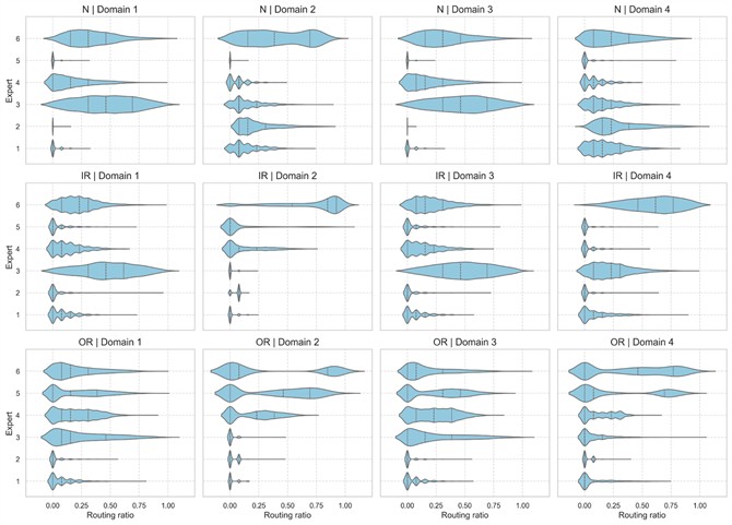
– Expert selection. To further understand the expert selection across different health states and different working conditions, we record the router selection corresponding to the top 10 % salient features within the dominant band of each sample, and calculate the expert routing ratio for each state-domain pair. The distributions of routing ratio for P1+P3+P4→P2 are visualized as an example in Fig. 12. We observed that salient features of different samples are extracted by different experts, and experts show specialization for different health states and different working conditions. In detail, we see: (1) adaptivity across working conditions: the distributions and emphasis of expert's routing ratio vary across different working conditions, where similar working conditions (Domain 1 and Domain 3) exhibit similar routing distribution, whereas distinct working conditions (Domain 2 and Domain 4) present markedly different expert routing distributions and emphasis, which indicates the model's adaptive routing under different working conditions; (2) expert specialization: inner race fault is primarily attended by expert 3 and 6, outer race fault is mainly attended by expert 4, 5 and 6, while for the normal state, the expert assignments are more dispersed under different working conditions. The above analysis indicates that the MoE with a multi-view router extracts features for different samples adaptively.
Table 9Ablation of backbones
Backbone | FFN | MoE w/o multi-view router | MoE w/ multi-view router | |
Accuracy (%) | Case 1: C2+C3+C4→C1 | 97.24±2.49 | 98.12±2.22 | 98.68±1.14 |
Case 2: P1+P3+P4→P2 | 92.12±2.78 | 92.61±1.48 | 94.25±2.11 | |
Case 3: H2+H3+H4→H1 | 84.67±6.04 | 90.16±4.59 | 96.74±0.97 | |
Fig. 12Distribution of routing ratios on three health states and four domains of case 2: P1+P3+P4→P2
– Runtime evaluation. Table 10 presents the runtime/performance evaluation of our model on case 2: P1+P3+P4→P2, including FLOPs (floating point operations per second), params (number of parameters), memory usage (sum of parameter storage and intermediate activations during forward inference), latency, and accuracy. Our model has 39.22M FLOPs and 0.15M parameters, requiring 394 MB of memory (388 MB for parameters and 6.7 MB for activations). It achieves 10.06 ms latency in a single forward pass and the highest accuracy of 94.25 % in this case. The low FLOPs and the small number of parameters indicate low computational requirements, while the MoE-based design leads to a relatively high static memory usage but an average-level activation memory during inference. The latency is also acceptable for practical applications. Overall, our model demonstrates low computational requirements and high performance.
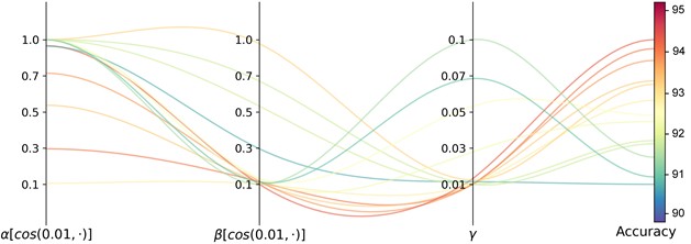
Sensitivity analysis of hyperparameters. In the proposed method, the model itself involves two hyperparameters: the number of experts and the number of selected top experts . Fig. 13 shows the results of different combinations of and on case 2: P1+P3+P4→P2. It can be observed that the proposed model performs well with TOP-1 expert when the number of experts is 6, 8, 10 and 16. However, the performance degrades significantly when the ratio of activated experts is high, as the specialization of each expert is weakened. In addition, the memory demand is increasing following with the number of experts. In the optimization strategy, there are three balancing parameters: for expert balancing, for monotonicity regularization and for sparsity regularization. To focus on the main task in the early stage of training, we update and with a cosine strategy from low to high. In contrast, is set a fixed one to maintain a fixed regularization to keep the model from learning spurious features. Fig. 14 shows the test accuracy during training for the controlled experiments on these three parameters on case 2: P1+P3+P4→P2. The proposed strategy, with updating from 0.01 to 1.0, updating from 0.01 to 0.1 and fixed at 0.01, achieves relatively high accuracy.
Table 10Runtime/performance comparison on case 2: P1+P3+P4→P2
Model | FLOPs (M) | Params (M) | Memory (MB) | Latency (ms) | Accuracy (%) |
WhiteningNet | 109.41 | 0.72 | 2.75+2.78 | 1.08±0.01 | 62.78±4.29 |
DGNIS | 218.22 | 0.85 | 21.42+5.54 | 2.57+0.30 | 70.53±3.60 |
CDDG | 665.12 | 1.10 | 4.20+9.46 | 3.67±0.57 | 64.18±1.28 |
ACRLN | 429.45 | 2.82 | 11.01+31.87 | 7.23±1.04 | 56.56±2.28 |
CIMSDG | 6.11 | 0.03 | 0.38+2.12 | 1.82±0.29 | 72.41±1.39 |
Ours | 39.22 | 0.15 | 387.59+6.72 | 10.06±0.30 | 94.25±1.72 |
Fig. 13Sensitivity of number of experts E and the number of selected top experts k on case 2: P1+P3+P4→P2
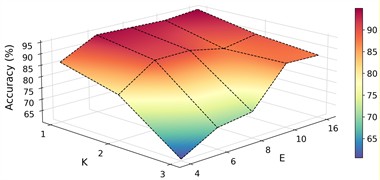
a) Performance
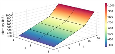
b) Memory
Fig. 14Sensitivity of balancing parameters α, β and γ on case 2: P1+P3+P4→P2
6. Conclusions
In this work, we propose a novel rolling bearing fault diagnosis method under the cross-working condition setting. The proposed approach, developed from the perspective of causality purification in a frequency band-aware manner, consists of three stages: cyclostationarity-enhanced representation generation, cycle frequency-level adaptive feature extraction via a mixture-of-experts (MoE) block with a multi-view router and a prior-knowledge-guided feature enhancer, and frequency band-level causal localization using a tokenized Transformer with an entropy-based sparsity regularization. Experiments demonstrate that the proposed model achieves good generalization performance in cases of working-condition transfer with distribution gaps ranging from small to large. In addition, the model provides good interpretability in the view of frequency band and cycle frequency.
While the proposed model demonstrates satisfactory performance under unseen working conditions, its performance highly depends on the quality of frequency band decomposition. Frequency bands obtained through wavelet packets decomposition may retain noise or irrelevant components. More advanced decomposition is the key to further motivating the potential of the model. In addition, the model relies on sufficient class-balanced data for training. As for future directions, it is necessary to investigate more efficient, lightweight, and transparent feature extraction mechanisms in the class-imbalanced case, including leveraging techniques such as knowledge distillation to lower deployment cost and self-supervised learning to alleviate the data imbalance constraint. These development directions are expected to facilitate the development of data-driven rolling bearing fault diagnosis algorithms in real-world applications.
References
-
L. Wen, X. Li, L. Gao, and Y. Zhang, “A new convolutional neural network-based data-driven fault diagnosis method,” IEEE Transactions on Industrial Electronics, Vol. 65, No. 7, pp. 5990–5998, Jul. 2018, https://doi.org/10.1109/tie.2017.2774777
-
H. Shao, H. Jiang, H. Zhao, and F. Wang, “A novel deep autoencoder feature learning method for rotating machinery fault diagnosis,” Mechanical Systems and Signal Processing, Vol. 95, pp. 187–204, Oct. 2017, https://doi.org/10.1016/j.ymssp.2017.03.034
-
Z. Chen and W. Li, “Multisensor Feature fusion for bearing fault diagnosis using sparse autoencoder and deep belief network,” IEEE Transactions on Instrumentation and Measurement, Vol. 66, No. 7, pp. 1693–1702, Jul. 2017, https://doi.org/10.1109/tim.2017.2669947
-
F. Wu et al., “Adversarial-causal representation learning networks for machine fault diagnosis under unseen conditions based on vibration and acoustic signals,” Engineering Applications of Artificial Intelligence, Vol. 139, p. 109550, Jan. 2025, https://doi.org/10.1016/j.engappai.2024.109550
-
N. Rezazadeh, M. de Oliveira, G. Lamanna, D. Perfetto, and A. de Luca, “WaveCORAL-DCCA: a scalable solution for rotor fault diagnosis across operational variabilities,” Electronics, Vol. 14, No. 15, p. 3146, Aug. 2025, https://doi.org/10.3390/electronics14153146
-
J. Wang et al., “Generalizing to unseen domains: a survey on domain generalization,” IEEE Transactions on Knowledge and Data Engineering, Vol. 35, No. 8, pp. 1–1, Jan. 2022, https://doi.org/10.1109/tkde.2022.3178128
-
Q. Li, L. Chen, L. Kong, D. Wang, M. Xia, and C. Shen, “Cross-domain augmentation diagnosis: An adversarial domain-augmented generalization method for fault diagnosis under unseen working conditions,” Reliability Engineering and System Safety, Vol. 234, p. 109171, Jun. 2023, https://doi.org/10.1016/j.ress.2023.109171
-
Y. Shi et al., “Domain augmentation generalization network for real-time fault diagnosis under unseen working conditions,” Reliability Engineering and System Safety, Vol. 235, p. 109188, Jul. 2023, https://doi.org/10.1016/j.ress.2023.109188
-
Y. Ding, M. Jia, Y. Cao, P. Ding, X. Zhao, and C.-G. Lee, “Domain generalization via adversarial out-domain augmentation for remaining useful life prediction of bearings under unseen conditions,” Knowledge-Based Systems, Vol. 261, p. 110199, Feb. 2023, https://doi.org/10.1016/j.knosys.2022.110199
-
Z. Shi, J. Chen, Y. Zi, K. Cao, and B. Li, “Semi-physical simulation-driven contrastive decoupling net for intelligent fault diagnosis of unseen machines under varying speed,” Measurement Science and Technology, Vol. 35, No. 7, p. 076101, Jul. 2024, https://doi.org/10.1088/1361-6501/ad36da
-
B. Pang, Q. Liu, Z. Xu, Z. Sun, Z. Hao, and Z. Song, “Fault vibration model driven fault-aware domain generalization framework for bearing fault diagnosis,” Advanced Engineering Informatics, Vol. 62, p. 102620, Oct. 2024, https://doi.org/10.1016/j.aei.2024.102620
-
X. Wang, H. Jiang, T. Zeng, and Y. Dong, “An adaptive fused domain-cycling variational generative adversarial network for machine fault diagnosis under data scarcity,” Information Fusion, Vol. 126, p. 103616, Feb. 2026, https://doi.org/10.1016/j.inffus.2025.103616
-
G. Zhang, X. Kong, H. Ma, Q. Wang, J. Du, and J. Wang, “Dual disentanglement domain generalization method for rotating Machinery fault diagnosis,” Mechanical Systems and Signal Processing, Vol. 228, p. 112460, Apr. 2025, https://doi.org/10.1016/j.ymssp.2025.112460
-
K. Xu, S. Li, S. Xu, Y. Hu, Y. Mao, and Y. Chai, “Mutual information-guided domain-shared feature learning for bearing fault diagnosis under unknown conditions,” IEEE Transactions on Instrumentation and Measurement, Vol. 74, pp. 1–12, Jan. 2025, https://doi.org/10.1109/tim.2025.3552003
-
Y. Dong, H. Jiang, Y. Liu, and Z. Yi, “Global wavelet-integrated residual frequency attention regularized network for hypersonic flight vehicle fault diagnosis with imbalanced data,” Engineering Applications of Artificial Intelligence, Vol. 132, p. 107968, Jun. 2024, https://doi.org/10.1016/j.engappai.2024.107968
-
C. Zhao and W. Shen, “A domain generalization network combing invariance and specificity towards real-time intelligent fault diagnosis,” Mechanical Systems and Signal Processing, Vol. 173, p. 108990, Jul. 2022, https://doi.org/10.1016/j.ymssp.2022.108990
-
Y. Xiao, H. Shao, J. Wang, B. Cai, and B. Liu, “Domain-augmented meta ensemble learning for mechanical fault diagnosis from heterogeneous source domains to unseen target domains,” Expert Systems with Applications, Vol. 259, p. 125345, Jan. 2025, https://doi.org/10.1016/j.eswa.2024.125345
-
F. Yue and Y. Wang, “Cross-domain fault diagnosis via meta-learning-based domain generalization,” in 2022 IEEE 18th International Conference on Automation Science and Engineering (CASE), pp. 1826–1832, Aug. 2022, https://doi.org/10.1109/case49997.2022.9926497
-
Y. Gao, J. Qi, Y. Sun, X. Hu, Z. Dong, and Y. Sun, “Industrial process fault diagnosis based on feature enhanced meta-learning toward domain generalization scenarios,” Knowledge-Based Systems, Vol. 289, p. 111506, Apr. 2024, https://doi.org/10.1016/j.knosys.2024.111506
-
M. Mu, H. Jiang, X. Wang, and Y. Dong, “A task-oriented theil index-based meta-learning network with gradient calibration strategy for rotating machinery fault diagnosis with limited samples,” Advanced Engineering Informatics, Vol. 62, p. 102870, Oct. 2024, https://doi.org/10.1016/j.aei.2024.102870
-
J. Li, Y. Wang, Y. Zi, and Z. Zhang, “Whitening-net: a generalized network to diagnose the faults among different machines and conditions,” IEEE Transactions on Neural Networks and Learning Systems, Vol. 33, No. 10, pp. 5845–5858, Oct. 2022, https://doi.org/10.1109/tnnls.2021.3071564
-
L. Cheng, X. Kong, Y. Zhang, Y. Zhu, H. Qi, and J. Zhang, “A novel causal feature learning-based domain generalization framework for bearing fault diagnosis with a mixture of data from multiple working conditions and machines,” Advanced Engineering Informatics, Vol. 62, p. 102622, Oct. 2024, https://doi.org/10.1016/j.aei.2024.102622
-
C. Guo et al., “CIS2N: Causal independence and sparse shift network for rotating machinery fault diagnosis in unseen domains,” Reliability Engineering and System Safety, Vol. 251, p. 110381, Nov. 2024, https://doi.org/10.1016/j.ress.2024.110381
-
Q. Guo, G. Li, and J. Lin, “A domain generalization network exploiting causal representations and non-causal representations for three-phase converter fault diagnosis,” IEEE Transactions on Instrumentation and Measurement, Vol. 73, pp. 1–13, Jan. 2024, https://doi.org/10.1109/tim.2024.3369153
-
L. Jia, T. W. S. Chow, and Y. Yuan, “Causal disentanglement domain generalization for time-series signal fault diagnosis,” Neural Networks, Vol. 172, p. 106099, Apr. 2024, https://doi.org/10.1016/j.neunet.2024.106099
-
Y. Zhu, Y. Zi, J. Li, and J. Xu, “PhysiCausalNet: a causal – and physics-driven domain generalization network for cross-machine fault diagnosis of unseen domain,” IEEE Transactions on Industrial Informatics, Vol. 20, No. 6, pp. 8488–8498, Jun. 2024, https://doi.org/10.1109/tii.2024.3369240
-
H. Ma, J. Wei, G. Zhang, X. Kong, and J. Du, “Causality-inspired multi-source domain generalization method for intelligent fault diagnosis under unknown operating conditions,” Reliability Engineering and System Safety, Vol. 252, p. 110439, Dec. 2024, https://doi.org/10.1016/j.ress.2024.110439
-
C. Guo, Y. Sun, R. Yu, and X. Ren, “Deep causal disentanglement network with domain generalization for cross-machine bearing fault diagnosis,” IEEE Transactions on Instrumentation and Measurement, Vol. 74, pp. 1–16, Jan. 2025, https://doi.org/10.1109/tim.2025.3545703
-
S. Jia, Y. Li, X. Wang, D. Sun, and Z. Deng, “Deep causal factorization network: A novel domain generalization method for cross-machine bearing fault diagnosis,” Mechanical Systems and Signal Processing, Vol. 192, p. 110228, Jun. 2023, https://doi.org/10.1016/j.ymssp.2023.110228
-
J. Li, Y. Wang, Y. Zi, H. Zhang, and C. Li, “Causal consistency network: a collaborative multimachine generalization method for bearing fault diagnosis,” IEEE Transactions on Industrial Informatics, Vol. 19, No. 4, pp. 5915–5924, Apr. 2023, https://doi.org/10.1109/tii.2022.3174711
-
J. Li, Y. Wang, Y. Zi, H. Zhang, and Z. Wan, “Causal disentanglement: a generalized bearing fault diagnostic framework in continuous degradation mode,” IEEE Transactions on Neural Networks and Learning Systems, Vol. 34, No. 9, pp. 6250–6262, Sep. 2023, https://doi.org/10.1109/tnnls.2021.3135036
-
Y. Liu, S. Zhou, X. Liu, C. Hao, B. Fan, and J. Tian, “Unbiased faster r-cnn for single-source domain generalized object detection,” in IEEE/CVF Conference on Computer Vision and Pattern Recognition (CVPR), pp. 28838–28847, Jun. 2024, https://doi.org/10.1109/cvpr52733.2024.02724
-
M. Xu, L. Qin, W. Chen, S. Pu, and L. Zhang, “Multi-view adversarial discriminator: mine the non-causal factors for object detection in unseen domains,” in 2023 IEEE/CVF Conference on Computer Vision and Pattern Recognition (CVPR), pp. 8103–8112, Jun. 2023, https://doi.org/10.1109/cvpr52729.2023.00783
-
J. Antoni, “Cyclostationarity by examples,” Mechanical Systems and Signal Processing, Vol. 23, No. 4, pp. 987–1036, May 2009, https://doi.org/10.1016/j.ymssp.2008.10.010
-
B. Li et al., “Sparse mixture-of-experts are domain generalizable learners,” in The Eleventh International Conference on Learning Representations, 2023.
-
X. Li, W. Zhang, H. Ma, Z. Luo, and X. Li, “Domain generalization in rotating machinery fault diagnostics using deep neural networks,” Neurocomputing, Vol. 403, pp. 409–420, Aug. 2020, https://doi.org/10.1016/j.neucom.2020.05.014
-
H. Zheng, R. Wang, Y. Yang, Y. Li, and M. Xu, “Intelligent fault identification based on multisource domain generalization towards actual diagnosis scenario,” IEEE Transactions on Industrial Electronics, Vol. 67, No. 2, pp. 1293–1304, Feb. 2020, https://doi.org/10.1109/tie.2019.2898619
-
R. Hu, M. Zhang, X. Meng, and Z. Kang, “Deep subdomain generalisation network for health monitoring of high-speed train brake pads,” Engineering Applications of Artificial Intelligence, Vol. 113, p. 104896, Aug. 2022, https://doi.org/10.1016/j.engappai.2022.104896
-
T. Han, Y.-F. Li, and M. Qian, “A hybrid generalization network for intelligent fault diagnosis of rotating machinery under unseen working conditions,” IEEE Transactions on Instrumentation and Measurement, Vol. 70, pp. 1–11, Jan. 2021, https://doi.org/10.1109/tim.2021.3088489
-
B. Wang, L. Wen, X. Li, and L. Gao, “Adaptive class center generalization network: a sparse domain-regressive framework for bearing fault diagnosis under unknown working conditions,” IEEE Transactions on Instrumentation and Measurement, Vol. 72, pp. 1–11, Jan. 2023, https://doi.org/10.1109/tim.2023.3273659
-
M. Arjovsky, L. Bottou, I. Gulrajani, and D. Lopez-Paz, “Invariant risk minimization,” in arXiv:1907.02893, Jan. 2019, https://doi.org/10.48550/arxiv.1907.02893
-
Z. Mo, Z. Zhang, Q. Miao, and K.-L. Tsui, “Sparsity-constrained invariant risk minimization for domain generalization with application to machinery fault diagnosis modeling,” IEEE Transactions on Cybernetics, Vol. 54, No. 3, pp. 1547–1559, Mar. 2024, https://doi.org/10.1109/tcyb.2022.3223783
-
D. Mahajan, S. Tople, and A. Sharma, “Domain generalization using causal matching,” arXiv:2006.07500, Jan. 2020, https://doi.org/10.48550/arxiv.2006.07500
-
Z. Sun, X. Zhu, J. Liu, X. Zhao, H. Wang, and R. Zhang, “A causality-inspired capsule network for domain generalization in cross-domain fault diagnosis of rolling bearing,” IEEE Transactions on Instrumentation and Measurement, Vol. 74, pp. 1–10, Jan. 2025, https://doi.org/10.1109/tim.2025.3569920
-
Y. Xie, G. Yang, H. Chen, Z. Zhao, and X. Leng, “Invariant feature purification method for domain generalization of rolling bearing fault diagnosis,” IEEE Transactions on Instrumentation and Measurement, Vol. 74, pp. 1–11, Jan. 2025, https://doi.org/10.1109/tim.2024.3522623
-
R. B. Randall and J. Antoni, “Rolling element bearing diagnostics-A tutorial,” Mechanical Systems and Signal Processing, Vol. 25, No. 2, pp. 485–520, Feb. 2011, https://doi.org/10.1016/j.ymssp.2010.07.017
-
I. Antoniadis and G. Glossiotis, “Cyclostationary analysis of rolling-element bearing vibration signals,” Journal of Sound and Vibration, Vol. 248, No. 5, pp. 829–845, Dec. 2001, https://doi.org/10.1006/jsvi.2001.3815
-
S. Zhou, D. Chen, J. Pan, J. Shi, and J. Yang, “Adapt or perish: adaptive sparse transformer with attentive feature refinement for image restoration,” in IEEE/CVF Conference on Computer Vision and Pattern Recognition (CVPR), pp. 2952–2963, Jun. 2024, https://doi.org/10.1109/cvpr52733.2024.00285
-
Z. Abidin, A. I. Mahyuddin, and W. Kurniawan, “Rolling bearing damage detection at low speed using vibration and shock pulse measurements,” ASEAN Engineering Journal, Vol. 4, No. 2, pp. 6–21, Aug. 2014, https://doi.org/10.11113/aej.v4.15417
-
X. Chen et al., “TimeMIL: advancing multivariate time series classification via a time-aware multiple instance learning,” in Proceedings of the 41st International Conference on Machine Learning, pp. 7190–7206, 2024.
-
Y. Xiong et al., “Nyströmformer: a Nyström-based algorithm for approximating self-attention,” arXiv:2102.03902, Jan. 2021, https://doi.org/10.48550/arxiv.2102.03902
-
T. Yan, D. Wang, S. Sun, C. Shen, and Z. Peng, “Novel sparse representation degradation modeling for locating informative frequency bands for Machine performance degradation assessment,” Mechanical Systems and Signal Processing, Vol. 179, p. 109372, Nov. 2022, https://doi.org/10.1016/j.ymssp.2022.109372
-
B. Wu, Y. Gao, S. Feng, and T. Chanwimalueang, “Sparse optimistic based on Lasso-LSQR and minimum entropy de-convolution with FARIMA for the remaining useful life prediction of machinery,” Entropy, Vol. 20, No. 10, p. 747, Sep. 2018, https://doi.org/10.3390/e20100747
-
X. Zhou, Y. Lin, W. Zhang, and T. Zhang, “Sparse invariant risk minimization,” in 39th International Conference on Machine Learning (ICML), pp. 27222–27244, 2022.
-
K. Zhang, S. Xie, I. Ng, and Y. Zheng, “Causal representation learning from multiple distributions: a general setting,” arXiv:2402.05052, Jan. 2024, https://doi.org/10.48550/arxiv.2402.05052
-
C. E. Shannon, “A mathematical theory of communication,” Bell System Technical Journal, Vol. 27, No. 3, pp. 379–423, Jul. 2013, https://doi.org/10.1002/j.1538-7305.1948.tb01338.x
-
W. A. Smith and R. B. Randall, “Rolling element bearing diagnostics using the Case Western Reserve University data: A benchmark study,” Mechanical Systems and Signal Processing, Vol. 64-65, pp. 100–131, Dec. 2015, https://doi.org/10.1016/j.ymssp.2015.04.021
-
C. Lessmeier, J. K. Kimotho, D. Zimmer, and W. Sextro, “Condition monitoring of bearing damage in electromechanical drive systems by using motor current signals of electric motors: A benchmark data set for data-driven classification,” in PHM Society European Conference, Vol. 3, No. 1, pp. 282–292, Jul. 2016, https://doi.org/10.36001/phme.2016.v3i1.1577
-
L. Hou et al., “Inter-shaft bearing fault diagnosis based on aero-engine system: a benchmarking dataset study,” Journal of Dynamics, Monitoring and Diagnostics, Vol. 2, No. 4, pp. 228–242, Aug. 2023, https://doi.org/10.37965/jdmd.2023.314
-
H. Zheng, Y. Yang, J. Yin, Y. Li, R. Wang, and M. Xu, “Deep domain generalization combining a priori diagnosis knowledge toward cross-domain fault diagnosis of rolling bearing,” IEEE Transactions on Instrumentation and Measurement, Vol. 70, pp. 1–11, Jan. 2021, https://doi.org/10.1109/tim.2020.3016068
-
J. K. Kimotho and W. Sextro, “An approach for feature extraction and selection from non-trending data for machinery prognosis,” in PHM Society European Conference, Vol. 2, No. 1, pp. 1–8, Jul. 2014, https://doi.org/10.36001/phme.2014.v2i1.1462
About this article

This work was supported in part by the Shanghai Pudong New Area Science and Technology Development Fund Public Welfare Scientific Research Project grant PKJ2025C08.
The datasets generated during and/or analyzed during the current study are available from the corresponding author on reasonable request.
Youlong Zhang: conceptualization, data curation, formal analysis, investigation, methodology, validation, visualization, writing-original draft preparation, writing-review and editing. Shan Jiang: resources, supervision, writing-review and editing. Wenrui Wang: resources, supervision. Jianfeng Yu: supervision. Fanglin Lu: supervision. Bo Wu: funding acquisition, supervision, writing-review and editing.
The authors declare that they have no conflict of interest.
