Abstract
Aiming at the problem of limited accuracy in motor bearing fault prediction under low-frequency, low-dimensional, and imbalanced data scenarios, this paper proposes a motor bearing fault early warning model based on a temporal convolutional network that integrates multi-attention mechanisms. The model leverages these mechanisms to enhance the network's ability to model long-term dependencies and focus on critical fault features from sparse data. To validate its performance, ablation and comparative experiments were conducted on a dataset of 10,000 samples collected from a self-built test bench. The experiment results demonstrate the superiority of the proposed model. Specifically, the Multi-Attention Temporal Convolutional Network achieved a coefficient of determination of 0.9629 and a Mean Absolute Error of 0.0244, significantly outperforming the standard Temporal Convolutional Network baseline which only achieved a Mean Absolute Error of 0.1349. These results indicate the excellent performance of the proposed model in this specific data prediction scenario, providing an effective solution to practical engineering problems where high-precision sensing equipment is unavailable.
Highlights
- A motor bearing fault early warning model (MA-TCN) integrating multi-attention mechanisms and TCN is proposed, which solves the problem of low prediction accuracy under low-frequency, low-dimensional and imbalanced data scenarios.
- The model fuses cross-attention, squeeze-and-excitation and temporal pattern attention, enhancing long-term dependency modeling and critical fault feature extraction from sparse data.
- Electromechanical fusion derived features are constructed to improve data representation under low-dimensional sensing, providing a practical solution for industrial low-cost sensor monitoring scenarios.
1. Introduction
In modern industrial settings, three-phase asynchronous motors have garnered significant attention due to their superior performance and wide-ranging applications. Among their components, bearings serve as the core elements enabling motor rotation, and their health status is critical to the stable operation of the entire mechanical system. However, even under normal conditions and when operating within predetermined parameters, bearings remain susceptible to various forms of damage. Over time, bearings are susceptible to a series of failures triggered by factors such as load, fatigue, insufficient lubrication, and improper operating conditions. Consequently, bearing failure prediction technology [1] plays a vital role in ensuring normal operation.
Since early bearing failures occur during the incipient stage, contact surface damage is minimal and vibration impacts are relatively weak, resulting in subtle failure characteristics. Furthermore, influenced by the motor's operating environment[2-3] and excitation from multiple vibration sources, sensors inevitably encounter interference from other noise during signal acquisition. This leads to a low proportion of failure-related components within the vibration signal, and operational failure data constitutes a small fraction of the total data volume. Consequently, such data is easily overlooked, allowing bearing damage to escalate.
Traditional bearing fault diagnosis methods such as singular value decomposition [4], empirical mode decomposition [5, 6], and wavelet packet transform [7, 8] process signals manifesting in various forms – vibration, temperature, sound, etc. – during fault occurrence. These methods extract characteristic components for fault identification. However, they suffer from weaknesses including limited capability for extracting deep, complex features, susceptibility to environmental influences, and reliance on prior information [9-11]. With advancements in fault diagnosis technology, intelligent analysis has emerged leveraging neural networks' robust data processing and learning capabilities. For instance, Wang Zhaowei et al. [12] employed parallel dilated convolutions to extract multi-scale features, combining adaptive selection to enhance the accuracy of improved convolutional networks. Jian Xianzhong et al. [13] proposed a novel lightweight bearing fault diagnosis network that generates high-quality samples, addressing issues such as excessive parameters and model complexity in traditional diagnostic methods under imbalanced data conditions. Liu Jun et al. [14] developed a rolling bearing fault diagnosis model integrating multi-branch convolutional networks and attention mechanisms. This approach converts time-domain signals into multi-domain features via convolutional networks, reducing feature extraction difficulty under strong noise. Attention mechanisms focus on fault feature maps, enhancing feature representation capabilities. Zhao Dengfeng et al. [15] employed BiLSTM to extract temporal bidirectional correlation features from input sequences. By introducing an attention mechanism to assign greater weight to critical spatio-temporal point features and integrating these into a convolutional neural network, they addressed the challenge of low fault diagnosis accuracy when training sample data is insufficient.
Although the aforementioned methods have achieved significant results in feature extraction and key feature focusing, previous research has largely focused on unified training using large-scale datasets composed of extensive high-frequency data [16-18]. This approach often overlooks data collected by low-frequency, low-cost, and lower-precision sensors employed in improvements on existing motor units due to cost constraints. In datasets with fewer data types and low fault sample ratios in time-series data [19, 20], it remains challenging to capture deep semantic information in low-dimensional spaces. Unbalanced samples can cause traditional models to favor the majority class, leading to limitations in diagnostic accuracy [21].
Therefore, this paper identifies a critical research gap: while numerous advanced bearing fault diagnosis models have been reported, most are validated under high-frequency, high-dimensional datasets and often fail to perform reliably in practical industrial scenarios characterized by low-frequency, low-dimensional, and imbalanced data. To address this gap, we propose a novel diagnostic framework that synergistically integrates complementary information from multiple domains. The primary contribution of this work is a Multi-Attention Temporal Convolutional Network (MA-TCN), which integrates a Cross-Attention mechanism (CA) to model cross-domain dependencies, a Squeeze-and-Excitation mechanism (SE) to recalibrate channel-wise feature importance, and a Temporal Pattern Attention mechanism (TPA) to emphasize diagnostically informative time intervals. Combined with the long-term dependency modeling capability of Temporal Convolutional Network (TCN), the proposed approach provides an effective solution for bearing fault diagnosis under low-quality data conditions.
This paper is organized into seven sections. Section 1 introduces the research background and significance of the studied problem and summarizes the main contributions of this work. Section 2 analyzes the physical mechanisms of early bearing degradation and its low-frequency manifestations in electrical and mechanical signals, establishing the physical relationships between bearing degradation, active power, and three-axis displacement vibration. Section 3 presents the proposed MA-TCN, detailing the core principles of TCN, different attention mechanisms, and their collaborative integration for bearing fault diagnosis. Section 4 focuses on the correlation analysis among measured parameters and the construction of derived features to enhance data representation under low-dimensional sensing conditions. Section 5 describes the experimental setup, including the test bench configuration, fault injection procedures, and model parameter settings. Section 6 evaluates the proposed approach through comprehensive experiments, including validation of the effectiveness of derived features and attention mechanisms, ablation studies, and comparative experiments with existing methods. Finally, Section 7 concludes the paper and discusses the main findings and potential future work.
2. Early bearing degradation analysis based on electrical-mechanical fusion
Fusion monitoring of bearing degradation is conducted from two independent yet causally linked dimensions: the electrical domain and the mechanical domain. This monitoring framework is grounded in a fundamental physical principle: deterioration in bearing condition directly alters the mechanical system's dynamic characteristics while simultaneously forcing the motor to consume more electrical energy to maintain its set speed and load. This, in turn, generates observable effects on the electrical side.
Traditional methods in electrical systems often rely on spectral analysis of current and voltage. However, in low-frequency monitoring scenarios, single parameters are highly susceptible to grid voltage fluctuations, reactive components, and harmonic interference from inverters, resulting in a low signal-to-noise ratio and limited sensitivity to early bearing degradation. In contrast, active power represents the effective energy conversion associated with mechanical load and thus provides a more direct electrical manifestation of mechanical abnormalities. Under stable operating conditions, variations in active power can be expressed in terms of the bearing degradation state:
where, is the regulated angular speed, denotes the nominal load torque under healthy conditions, and represents the torque perturbation induced by the bearing degradation state . Consequently, trend monitoring based on active power intrinsically suppresses the influence of reactive components and harmonic distortions, effectively avoiding false alarms caused by grid fluctuations and normal process adjustments, and offering a reliable electrical-level validation for mechanical system anomalies.
Vibration analysis is the most direct method for bearing fault diagnosis, and the selection of displacement parameters is crucial for capturing low-frequency fault characteristics [22-24]. Early-stage bearing failures (e.g., pitting, wear) primarily alter the dynamic behavior of the rotor-bearing system, resulting in pronounced low-frequency vibration responses. The corresponding three-axis displacement vibration can be expressed as:
where, represents the degradation-dependent dynamic response of the mechanical system. Compared to velocity or acceleration, displacement parameters exhibit higher measurement sensitivity and signal-to-noise ratio for low-frequency vibration components. This characteristic allows low-frequency vibration energy to be preserved and amplified rather than attenuated during signal processing, thereby facilitating the extraction of the following critical fault-related characteristics:
– Axis trajectory variation: Wear, increased clearance, or surface damage in bearings leads to distorted, disordered trajectory patterns with expanding scope [25].
– Low-frequency shock: Local defects on raceway surfaces induce periodic low-frequency impacts. These transient impacts excite the natural vibrations of the rotor-bearing system, triggering periodic large-amplitude fluctuations:
where, from a unified physical perspective, bearing degradation can be abstracted as a common latent state governing both electrical and mechanical responses of the motor system. As the degradation state evolves, it induces low-frequency torque perturbations and alters the dynamic characteristics of the rotor-bearing system, which are jointly reflected in the electrical and mechanical domains as:
The above analysis establishes a unified physical interpretation in which bearing degradation acts as a common driving factor underlying both electrical and mechanical observations. This provides a clear theoretical foundation for subsequent feature correlation analysis and data fusion modeling, enabling the extraction of complementary degradation information from low-frequency, low-dimensional measurements.
3. Framework of TCN fault prediction model integrating multi-attention mechanisms
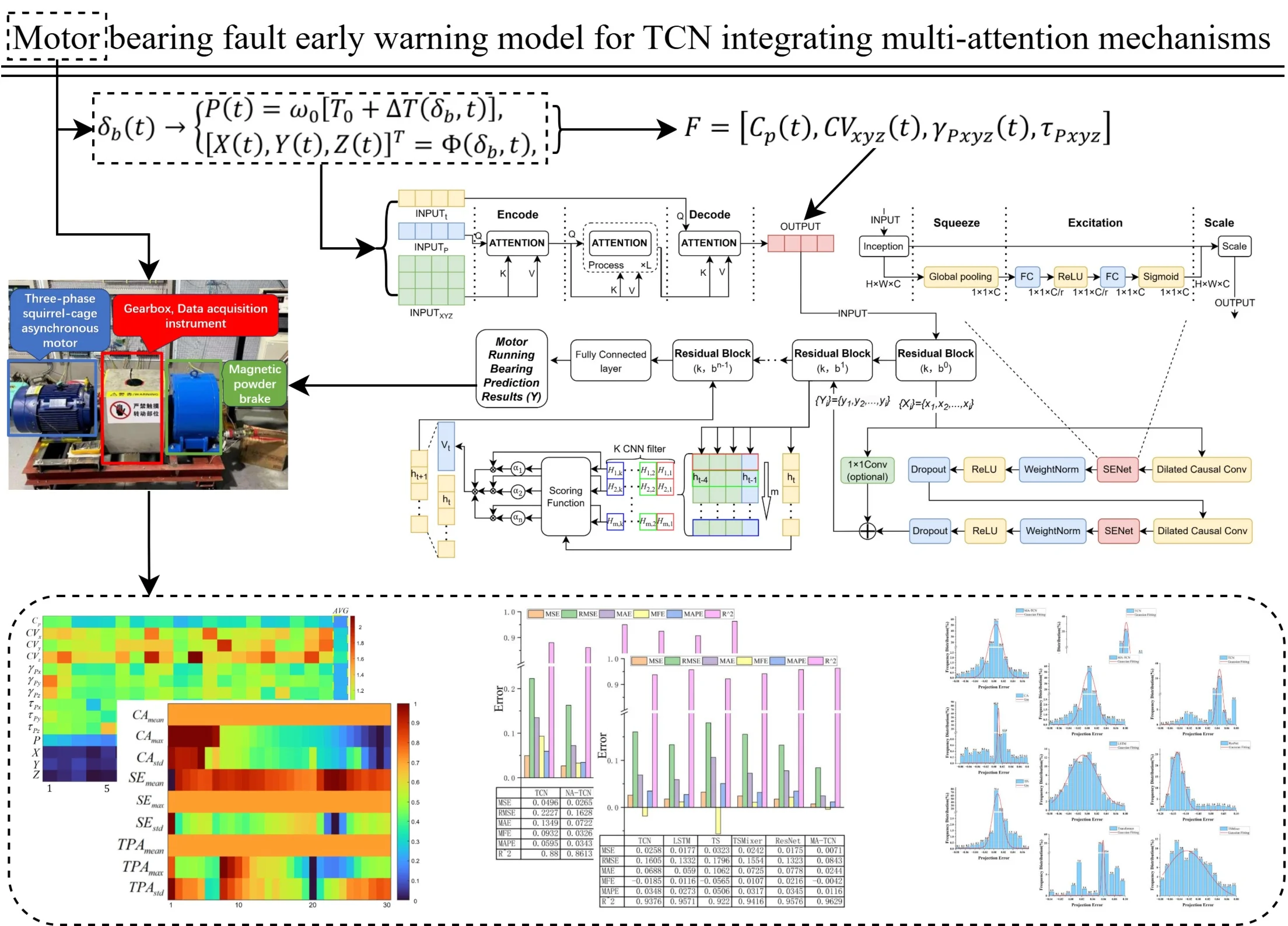
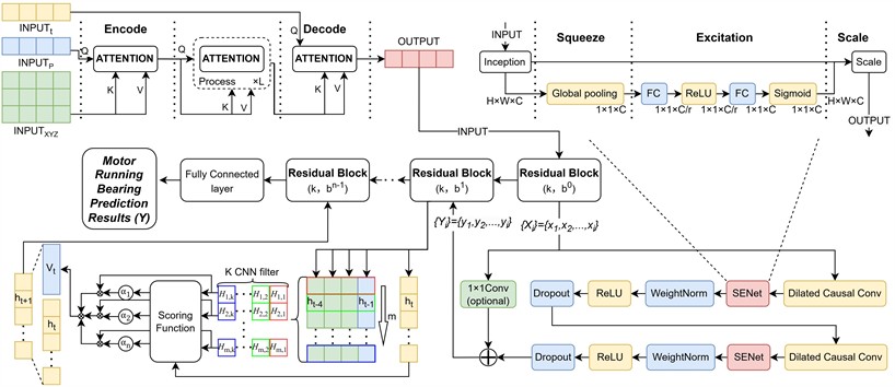
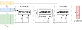
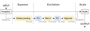
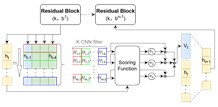
The algorithmic component of the proposed TCN-based multi-attention motor bearing fault prediction framework comprises a three-layer network. As illustrated in Fig. 1(a), the first layer employs a the CA to enhance feature fusion among parameters by considering their correlation with bearing faults [26, 27], enabling real-time derivative feature computation. The second layer combines a temporal convolutional neural with the SE. This effectively captures long-term temporal dependencies between multi-dimensional vibration variations and operational power. By introducing physical mechanism constraints that link faults to channel weight sensitivities, this integration enhances the representation of relevant input information within the TCN framework. The third layer employs a the TPA. By assigning different probability weights to the outputs of the TCN hidden layer, it enhances the predictive framework model [28, 29], This forces the model to focus on critical temporal segments where failures occur, thereby improving prediction accuracy.
Fig. 1Overall framework and key mechanisms of the MA-TCN model
a) Overall Framework of the MA-TCN Model
b) Cross-Attention mechanism
c) Squeeze-and-excitation mechanism
d) Temporal pattern attention mechanism
Using TCN as the foundational fault prediction model, to address the integration and temporal discrepancies between electrical and mechanical data within motor operational parameter inputs, and to enhance the network's predictive performance, a multi-attention mechanism is introduced. This incorporates CA on the input side during model training, comprehensively integrating electrical and mechanical data to uncover intrinsic correlations and focus on critical time intervals. Introducing SE into residual connections autonomously optimizes weight distribution after expanded causal convolutions, extracting raw features from motor bearing time series data. This identifies long-term dependencies between fault criteria and multidimensional vibration parameter features. Expanded causal convolutions address long historical sequence challenges, enabling cross-layer transmission of fault data information. Introducing TPA at the output layer extracts temporal relationships between historical data points, emphasizing information representation at critical time intervals.
3.1. Cross-attention mechanism
The core of the CA lies in enabling a query sequence to focus on another key-value sequence, capturing dependencies between input parameters to achieve information fusion. As shown in Fig. 1(b), the CA architecture takes time-series parameters , electrical parameters , and mechanical parameters as inputs.
To achieve this fusion, the input features are first projected into the three key components of the attention mechanism: the Query, Key, and Value matrices. Specifically, the temporal features are linearly transformed to generate the matrix. Simultaneously, the electrical features and mechanical features are concatenated and then jointly subjected to two separate linear transformations to produce the and matrices. These transformations are performed by learnable weight matrices, allowing the model to adaptively determine the optimal representation for querying and for being queried.
Once the , , and matrices are derived, the attention scores are computed according to Eq. (4). This process allows the temporal features as the query to selectively attend to the most salient information within the combined electrical and mechanical features as the key-value source. Through this mechanism, the model effectively fuses heterogeneous sensor data, enhancing its ability to learn from fault-related patterns that manifest across different data streams:
where, , and are the matrices derived from the input features , , and as described above. ⨂ denotes matrix multiplication. is a scaling factor based on the key dimension, and represents the Softmax function calculates the final attention weights.
3.2. Temporal convolutional neural network with the squeeze-and-excitation mechanism
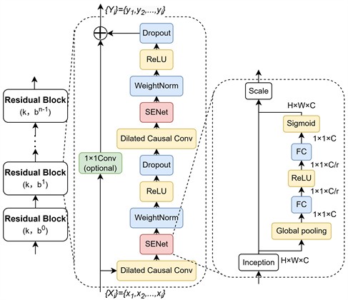
TCN can handle the strong temporal nature of motor operation data, addressing sequential issues during prediction while modeling dependencies in long-term [30] data within shorter timeframes. When combined with channel attention mechanisms, TCNs optimize weight distribution among data points, enabling greater focus on parameters with stronger simultaneous influence on faults. Their model structure is illustrated in Fig. 2.
The expansion causal convolutions and residual connections within the TCN effectively prevent gradient vanishing and overfitting. This ensures that the output at time t depends solely on the input data transmitted up to that point, avoiding confusion between historical and future information. By appropriately selecting the dilation factor and convolution kernel size, the model effectively processes long-term sequence information, expands the receptive field of network layers, and balances network depth and complexity, as detailed in Eq. (5):
where, denotes the filter function, represents the input data value shifted backward by time steps from time , and ∗ indicates the convolution operation.
Residual connections address the issue of gradient vanishing caused by the continuous stacking of network layers due to the enlarged receptive fields from dilated convolutions. They also enable cross-layer transmission of multi-dimensional data information, enhancing computational efficiency. Within the residual block, the sequence of operations is arranged as dilated causal convolution, channel attention, weight normalization, activation function, and random deactivation, as shown in Fig. 2. Incorporating the channel attention mechanism before weight normalization enhances inter-channel information exchange, adaptively adjusts weights across different channels, and simultaneously improves the model’s generalization capability. The residual block is defined by Eq. (6), and the SE is defined by Eq. (7):
where, denotes the ReLU activation function, represents the five-part transformation comprising dilated convolutions, channel attention, weight normalization, activation functions, and random deactivation. and represent the outputs of the th and th residual blocks, respectively. and represent the channel features before and after SE weighting, respectively. represents the global features for each channel. , are the weight matrices for dimensionality reduction and dimensionality augmentation operations. denotes the sigmoid activation function.
Fig. 2Temporal convolutional neural with the squeeze-and-excitation architecture
3.3. Temporal pattern attention mechanism
To enhance the stability of temporal modeling and amplify the features of incipient faults, a the TPA is introduced. As depicted in Fig. 1(d), a TPA layer is strategically inserted between each pair of consecutive residual blocks within the Temporal Convolutional Network architecture. This placement allows the model to iteratively refine its focus on critical temporal patterns as data flows through the network.
The function of each TPA layer is to re-weight the feature sequence it receives. Specifically, the input to a TPA layer is the complete feature sequence output by the preceding TCN residual block. The TPA layer then internally uses a set of one-dimensional convolutional filters to assess the importance of different temporal patterns across the entire sequence, generating an attention score for each time step.
These scores are normalized and used as weights to compute a weighted sum of the original input sequence, a process summarized by Eq. (8). The output of the TPA layer is this re-calibrated feature sequence, which has the same dimensions as the input. This output then serves directly as the input for the subsequent TCN residual block:
where, represents the hidden states from the input sequence, denotes the sigmoid activation function, represents the scoring function, denotes with the convolution kernel omitted, denotes matrix transposition, and denotes the learnable weight matrix. The resulting vector is the attention-optimized output sequence.
This iterative process of feature extraction by a TCN block and temporal re-weighting by a TPA layer) strengthens the model’s ability to capture subtle fault indicators over long sequences. The feature sequence from the final TPA layer is then passed to a fully connected layer to produce the ultimate motor bearing fault prediction .
4. Correlation analysis of bearing fault
Based on the physical relationships among motor parameters and their temporal variations under bearing fault conditions, the correlations and temporal dependencies among them are further investigated. A set of derived features is constructed to characterize the statistical dependency and temporal correlation between active power and vibration signals, thereby enhancing the effective data dimensionality.
4.1. Temporal fluctuation characteristics of active power under bearing failure
Active power serves as the core parameter reflecting a motor’s energy consumption and load status. When bearings are functioning normally, the rotor’s operational resistance remains stable. Under conditions where stator current, voltage, and power parameters are essentially constant, power generally maintains a steady range. The instantaneous active power , as derived from Eq. (9), corresponds to the average active power :
After power is supplied to the motor stator, electrical energy is first converted into electromagnetic power . However, this does not translate into mechanical power without losses, as stator-side losses must be considered. These primarily consist of stator copper losses and stator iron losses . For simplified analysis, stator iron losses can be temporarily neglected due to their small magnitude. Therefore, the stator power can be approximated as .
When bearing failure occurs, the electromagnetic torque becomes less than the load torque , causing the rotational speed n to inevitably decrease. Calculating the slip rate yields . With the synchronous speed remaining constant, this decrease in rotational speed leads to an increase in electromagnetic power, thereby driving up the average active power.
For low-frequency time-series data, it is necessary to characterize the power fluctuation patterns within the sliding window. Define the sliding window length as and the sliding step size as 1. For any time point corresponding to the sliding window, the active power data sequence it contains can be represented as .
The time span aligns with the periodic characteristics of low-frequency signals, enabling real-time capture of trend changes in low-frequency active power timing. The step size slides sequentially by data points to ensure no omissions, thereby quantifying fault features within the window. This can be expressed using Eqs. (10-11) [31]:
where, denotes the power variance within the window, and denotes the power mean within the window. is the coefficient of time-series fluctuation for active power. Used to distinguish between “normal fluctuations” and “fault fluctuations” in low-frequency time-series data, it suppresses interference from steady-state power amplitude variations under different operating conditions, reflecting the steady-state power level within the observation window.
4.2. Temporal statistical characteristics of three-axis displacement vibration under bearing failure
The , , and -axis vibration displacements are direct physical quantities reflecting the mechanical condition of the bearing. Their low-frequency time-series data encapsulate the macroscopic characteristics of rotor motion, better revealing the gradual progression of fault evolution compared to high-frequency signals. During normal operation, the and -axis radial vibrations maintain low-amplitude fluctuations due to the symmetrical rotation of the rotor, while the -axis axial vibration amplitude approaches zero. The time-series mean and standard deviation of all three axes remain within specified limits.
For low-frequency vibration data, the window design is consistent with that used in active power analysis. The data sequences it encompasses can be represented as . Taking -axis vibration as an example, the coefficient of variation is calculated to standardize the representation of vibration dispersion, thereby eliminating interference from variations in steady-state vibration amplitude across different operating conditions:
where, represents the standard deviation of the -axis vibration window, indicating the intensity of data fluctuations within that window. denotes the steady-state displacement baseline within the window.
4.3. Joint characterization of low-frequency fluctuations in bearing failure
Bearing failure fluctuations manifest as coupled variations in mechanical vibration and energy consumption, appearing in low-frequency time-series data as coordinated anomalies in active power and vibration displacement. During normal operation, stable mechanical resistance results in weak correlation between vibration and power fluctuations. Under fault conditions, sudden changes in mechanical impedance trigger strong coupled fluctuations. This state manifests as increased mechanical impedance disrupting torque balance, causing reduced rotational speed and increased slip rate. Consequently, average active power rises while three-axis vibration displacement exhibits abnormal fluctuations. Eq. (14) constructs characteristic vectors to comprehensively describe fault fluctuations:
Eq. (15) employs a sliding window Pearson correlation [32] to quantify the linear association strength between active power and -axis vibration displacement within the same time window. Similarly, and are obtained for the and axes, respectively, with correlation coefficients ranging between [–1, 1]. During normal operation, the mechanical system remains stable, and the Pearson correlation coefficient does not exhibit abnormal values near the boundary. Under fault conditions, periodic impacts cause highly synchronized trends in both variables, leading to a significant increase in the Pearson correlation coefficient. Moreover, abnormal peak values in a specific axis system can assist in locating the fault direction:
where, represents the maximum cross-correlation criterion [33], identifying the value that maximizes the summation term. Here, denotes the lag time, used to analyze the physical delay inherent in the power response transmitted through the rotor system during mechanical vibration impacts. Similarly, and are obtained for the and axes. During fault conditions, mechanical impact energy is transmitted through the bearing-stator winding to trigger power changes. Therefore, the vibration impact must precede the power variation.
5. Establishment of test benches and preparation for testing the TCN model with integrated multi-attention mechanisms
With the experimental platform established, this section details the comprehensive methodology used for model validation. The process begins with the artificial inducement of specific bearing faults to generate a representative dataset, followed by the configuration of the model's parameters and the definition of the evaluation criteria used to assess its performance.
5.1. Bearing failure simulation method
Based on core requirements for industrial operation and fault monitoring, the system focuses on two typical states:
1) Normal operation state: Utilizes identical healthy bearings to confirm the absence of mechanical faults in the motor, while acquiring baseline electrical and mechanical parameters.
2) Bearing fault state: Emulates actual failure scenarios using artificially prepared faulty bearings to analyze abnormal parameter variations under different load conditions. The artificially induced bearing faults, as shown in Fig. 3(a), include insufficient lubrication, surface scratches on individual rolling elements, scratches and dents on the inner ring, and irregular damage to the rolling element cage.
To cover common industrial load scenarios, motor loads were set to no-load, 30 %, 50 %, 70 %, and 100 %. Under each operating condition, the motor first ran stably for 30 minutes before collecting data in both normal and fault states, ensuring consistent comparison benchmarks between the two states. As shown in Fig. 3(b), the primary equipment includes a three-phase squirrel-cage induction motor, gearbox, data acquisition unit, and magnetic powder brake. The data sampling frequency was set to 1 Hz. The magnetic powder brake adjusted the load and connected to the motor via sensors and the gearbox. Motor parameters are detailed in Table 1.
Fig. 3Bearing fault state & IM fabricated test rig description
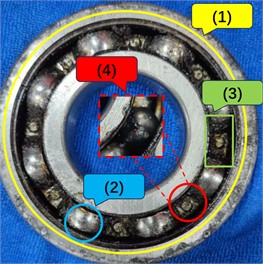
a) Bearing fault state: 1 – lubrication deficiency; 2 – rolling element surface scratches; 3 – cage irregular damage; 4 – inner ring scratches and dents
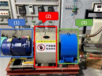
b) IM fabricated test rig: 1 – three-phase squirrel-cage asynchronous motor; 2 – gearbox, data acquisition instrument; 3 – magnetic powder brake
Table 1Basic size and style requirements
No | Parameters | Values |
1 | Rated power | 5.5 KW |
2 | Rated voltage | 380 V |
3 | Rated current | 11.2 A |
4 | Rated frequency | 50 Hz |
5 | Rated efficiency | 89.6 % |
6 | Power factor | 0.83 |
7 | Rated speed | 1465 r/min |
8 | Connection | Δ |
9 | Protection level | IP55 |
10 | Insulation level | F(155℃) |
Raw motor operating data is collected through the experimental platform. Under multiple operating conditions, non-steady-state data emerges during load gradient increases. The critical threshold for data stability is determined, and based on this, steady-state data outside this range is processed. The “3” criterion method is employed to detect and eliminate outliers. To prevent differing units and dimensions of various parameter characteristics from affecting fault prediction accuracy, preprocessed data undergoes MAX-MIN normalization. All parameters are mapped to the [0, 1] range eliminate the impact of dimensional differences between data features. The final dataset contains 10,000 bearing operational records. To ensure an unbiased evaluation, the dataset was partitioned into training, validation, and test sets using a 7:1.5:1.5 ratio through a stratified sampling methodology. The stratification was performed based on both the operating status (normal vs. fault) and the specific internal load condition of the fault data. This approach guarantees that the proportional representation of each category is preserved across all three sets, preventing evaluation bias and ensuring the model is tested on a representative distribution of the data, including rare fault conditions.
1) Operating Status: The overall ratio of normal to fault data is 74:26, which is maintained in the training, validation, and test sets.
2) Internal Motor Load Fault Data: Within the fault data, the distribution ratio for no-load, 30 %, 50 %, 70 %, and 100 % load conditions is 37:25:21:14:3, and this proportion is also consistently reflected in each dataset partition.
5.2. Model parameter configuration and evaluation criteria
The MA-TCN model was constructed within the PyTorch framework. Through debugging, the optimal iteration count was determined to be 100 with a batch size of 128. The bearing prediction model comprises a CA layer, TCN-SE layer, and TPA layer. Due to the integration of multiple attention mechanisms, network parameters are determined by the outputs of the preceding layers. Detailed parameter settings for each layer of the MA-TCN model are shown in Table 2.
Table 2MA-TCN parameter settings
Model | Parameter | Setup |
TCN | Dilation factor | [1, 2, 4, 8] |
Dropout | 0.05 | |
Kernel | 3 | |
Conv layer channels | [32, 64, 128, 256] | |
Activation function | ReLU | |
Optimizer | Adam | |
Learning rate | 0.00001 | |
Multiple layers of attention | Hidden layers | 4 |
Hidden units | 256 | |
CA layer output dimension | [16, 4, 128] | |
SE layer output dimension | [16, 256, 128] | |
TPA layer output dimension | [16, 256, 128] |
The key hyperparameters presented in Table 2 were determined through a systematic process of empirical tuning, guided by the model’s predictive performance on a validation set. This iterative approach allowed for the refinement of the architecture to best suit the specific characteristics of the bearing fault data. For the dilation factors, the sequence [1, 2, 4, 8] was established as the most effective configuration. Preliminary evaluations with shallower dilation structures (e.g., [1, 2, 4]) resulted in a diminished receptive field and, consequently, a degraded ability to model long-term dependencies, leading to poorer performance. The kernel size was set to 3 after observing that it provided the optimal balance between local feature extraction and computational load. While smaller kernels failed to capture sufficient temporal context, larger ones did not yield a corresponding performance gain, thus making 3 the most efficient choice. Similarly, the channel dimensions were fine-tuned through experimentation. We observed that increasing the channel depth from 64 to 128 allowed the model to learn more complex and abstract feature representations, which significantly improved prediction accuracy. However, further increases in channel width led to diminishing returns and increased the risk of overfitting. Therefore, the final configuration in Table 2 represents an empirically optimized balance between model capacity and generalization performance for this specific application.
For the convolutional layers, the channel configuration [32, 64, 128, 256] follows a progressive expansion scheme to enable hierarchical feature extraction. The shallow layers capture low-level temporal patterns, while deeper layers learn more abstract representations. This design ensures sufficient expressive capacity with manageable computational cost. In the attention modules, the output dimensions of the CA, SE, and TPA layers were set to [16, 4, 128], [16, 256, 128], and [16, 256, 128], respectively, to maintain compatibility with TCN feature dimensions and preserve key channel and temporal dependencies. These values strike a balance between model expressiveness and training stability, as excessively large or small dimensions degraded performance during preliminary tuning.
To systematically validate the performance of the MA-TCN model in predicting low-dimensional unbalanced parameters for motor bearing faults, this study adopts a comprehensive evaluation framework incorporating six metrics: MSE, RMSE, MAE, MFE, MAPE, and . Detailed calculation formulas for each metric are provided in Table 3.
Each tailored to address specific evaluative objectives for targeted model assessment:
– MSE: Sensitive to large errors, emphasizing significant deviations between predicted and actual values.
– RMSE: Reflects the actual error magnitude, providing an intuitive measure in the same unit as the original data.
– MAE: Captures the overall average error across all fault stages, enabling robust assessment of consistent performance throughout fault evolution.
– MFE: Identifies the model’s overall prediction bias, indicating tendencies toward overestimation or underestimation of fault parameters.
– MAPE: Compares relative accuracy across fault stages, supporting fair evaluation of relative deviations independent of the absolute magnitude of fault parameters.
– : Measures goodness of fit to bearing fault evolution trends, assessing the model’s ability to capture the intrinsic pattern of fault development.
Table 3MA-TCN prediction performance
No | Formula |
1 | |
2 | |
3 | |
4 | |
5 | |
6 |
Notably, MSE, RMSE, MAE, MFE, and MAPE quantify prediction deviations via absolute or relative error metrics – lower values (closer to 0) denote higher local prediction accuracy. evaluates the model’s ability to align with actual data trends, with values approaching 1 indicating superior overall fit. While these error metrics are computed on the normalized [0, 1] data scale, they possess direct practical engineering significance. Since the model's output is a normalized representation of physical parameters, the metrics quantify prediction error as a fraction of the sensors' full operational range. In an industrial context, a low error value (e.g., a low MAE) signifies high fidelity between the model's prediction and the system’s true physical state. This is critical for engineering applications, as it ensures the reliability of the fault warning system and allows for the confident setting of precise alarm thresholds for timely preventative maintenance.
6. Experimental results and model evaluation
This paper employs a combined analysis method of derivative feature validation, ablation, and comparative experiments, integrated with the aforementioned evaluation metrics, to comprehensively assess the effectiveness of the MA-TCN model in fault prediction under low-frequency, low-dimensional imbalanced data. Before conducting ablation and comparative experiments, an additional experiment is designed to validate the necessity of the derived features, ensuring that each constructed parameter contributes meaningfully to the model’s predictive performance. Ablation experiments progressively remove and modify key components within the model to validate the contribution of each module to overall performance. Comparative experiments select current mainstream models for cross-sectional comparison, demonstrating the superiority of this model under special sample data conditions.
6.1. Derivative feature validation experiment and attention mechanism activation analysis
To evaluate the necessity and contribution of the derived features, we conducted 20 repeated training runs of the MA-TCN model. For each run, the Permutation Importance of both the original parameters and the ten derived features was computed.
Fig. 4Derived feature contribution heatmap
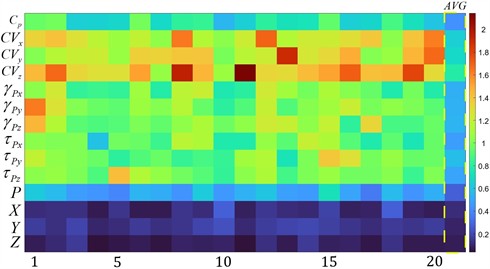
Fig. 4 presents the Derived Feature Contribution Heatmap, which provides a visual representation of feature importance across the 20 repeated MA-TCN runs. As shown in the heatmap, the derived features consistently exhibit higher importance than the original parameters, confirming their substantial contribution to the model’s predictive performance. In particular, the coefficients of variation demonstrate the most significant influence across nearly all runs, highlighting the effectiveness of capturing temporal-vibration fluctuation characteristics in supplementing the limited dimensionality of the original input data.
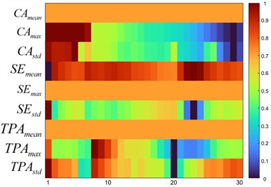
To validate the multi-attention architecture, we extracted activation patterns of its three core modules (CA, SE, TPA) from 30 test samples and computed three statistical metrics for each module. For each mechanism, three statistical metrics were computed: Mean (overall activation strength), Max (peak attention value), and Std (attention concentration degree).
Table 4 defines the nine attention indicators used in this analysis, detailing their definitions and physical interpretations within the MA-TCN.
Table 4Definition and physical interpretation of attention mechanism
Indicators | Definition | Physical interpretation |
The mean value of all elements in the attention matrix | Represents the overall intensity of cross-channel interactions when processing a given sample | |
The maximum value in the attention matrix | Indicates the strongest attention connection between two time steps or feature pairs | |
The standard deviation of all attention weights | Measures the degree of attention concentration | |
The mean of the 256 channel weights in the last TCN layer | Reflects the overall level of channel activation | |
The weight of the most important channel among 256 channels. | Quantifies the activation strength of the most discriminative feature channel | |
The standard deviation of the 256 channel weights | Measures the degree of differentiation in channel importance | |
The mean of attention weights across 128 time steps | Represents the baseline temporal attention level | |
The weight of the most attended time step among 128 time steps | Identifies the importance of the most critical temporal moment | |
The standard deviation of attention weights across 128 time steps | Measures the degree of temporal attention concentration |
Fig. 5 presents the Attention Mechanism Activation Heatmap, with each row representing a specific metric and each column corresponding to an individual test sample. The color intensity indicates normalized activation strength. Key observations include:
1) CA: exhibits variable values across samples 2-8, indicating adaptive learning of inter-feature correlations critical to fault identification.
2) SE: maintains consistently high activation, confirming robust channel recalibration, while variability in certain samples demonstrates the mechanism’s ability to differentiate channel importance based on fault characteristics.
3) TPA: shows pronounced peaks in specific samples 8-10, revealing successful identification of fault-critical time steps, which is essential for capturing transient anomalies in low-frequency data.
These complementary activation patterns confirm that the multi-attention architecture enables the MA-TCN model to effectively extract discriminative features from low-dimensional, imbalanced temporal data, validating the design rationale of integrating CA, SE, and TPA mechanisms.
Fig. 5Multi-attention mechanism contribution heatmap
6.2. Evaluation of ablation experiment results
The modified networks for the ablation experiments were TCN, NA-TCN (Non-Attention TCN), SE-TCN, CA-TCN, and TPA-TCN. These networks were trained under the same datasets, model configurations, and evaluation metrics as described above. The experimental evaluation results are shown in Figs. 6-7.
Fig. 6Evaluation results of different models in ablation experiments
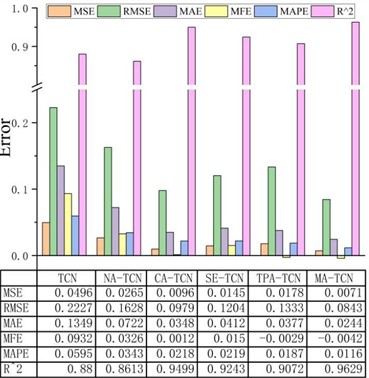
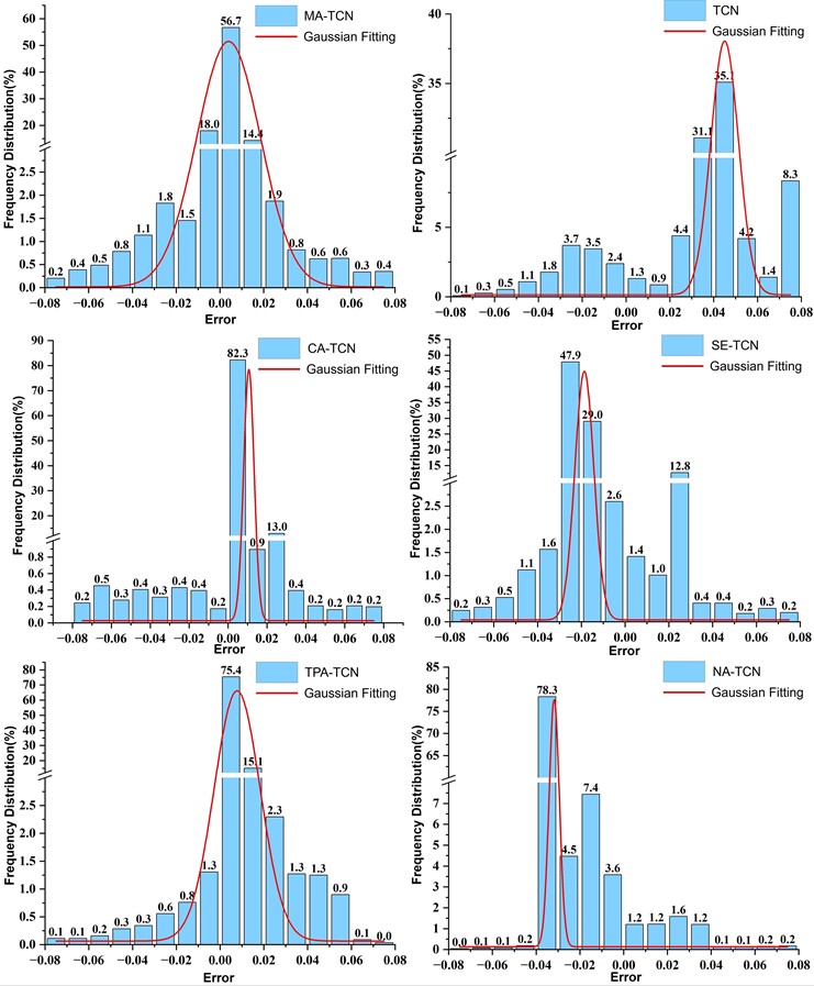
Fig. 7Histogram of the frequency distribution of model prediction errors in ablation experiments
As shown by the experimental results in Fig. 6, the performance of CA-TCN, SE-TCN, and TPA-TCN significantly outperforms that of TCN and NA-TCN. This result indicates that integrating attention mechanisms with TCN effectively enhances the model's ability to extract valuable information from data while suppressing interference from irrelevant information.
Specifically, compared to TCN and NA-TCN, the R² values of CA-TCN, SE-TCN, and TPA-TCN all show notable improvements. Among these, CA-TCN introduces a the CA mechanism on top of TCN, learning dependencies among inputs in the data similarly to derived data; SE-TCN implements a channel attention mechanism to redistribute weights for critical fault information within residual connections; TPA-TCN leverages temporal attention to enhance the capture of fault time periods.
Based on the above analysis, this paper effectively integrates multiple attention mechanisms to propose MA-TCN. Ablation experiments demonstrate that compared to models combining a single attention mechanism with TCN, MA-TCN – which combines multiple attention mechanisms with TCN – exhibits superior predictive performance on special data. Experimental results show that MA-TCN achieves optimal metrics across all evaluation indicators, with an value as high as 0.9629. Furthermore, comparing the error distributions across models in Fig. 7 reveals that MA-TCN exhibits a Gaussian distribution of prediction error frequencies. Its prediction errors converge to a narrow range, indicating high prediction accuracy. These evaluation metrics collectively validate the high consistency between MA-TCN's predictions and actual values, demonstrating the model's strong fitting capability for predicting low-frequency, low-dimensional imbalanced data.
6.3. Evaluation of comparison experiment results
To ensure a fair and rigorous comparison, all baseline models were implemented based on their well-established, publicly recognized architectures, and subsequently tuned for the specific task of bearing fault diagnosis. Specifically, the architectures for LSTM and Transformer were adapted from their seminal works [34-35], while the ResNet model utilized a one-dimensional adaptation of the canonical residual learning framework [36]. The more recent TSMixer baseline was implemented according to its original proposed structure [37].
For each of these models, a consistent empirical tuning process was applied, focusing on optimizing key hyperparameters such as the number of layers, hidden unit dimensions, and learning rate to ensure each model achieved a robust performance level on our dataset. This approach guarantees that the comparison is not merely against default configurations, but against strong, representative implementations of each baseline, thus providing a fair benchmark for evaluating our proposed MA-TCN model.
Fig. 8Evaluation results of different models in comparison experiments
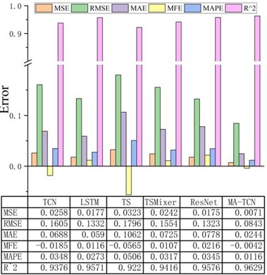
As observed in the prediction results of Fig. 8, similar to how LSTM leverages its gated recurrent feature to handle variable-length, non-uniformly sampled sequences, ResNet effectively mitigates the vanishing gradient problem in long sequence training through its fixed residual branch design. While LSTM achieves parameter sharing in the temporal dimension, ResNet accomplishes convolution kernel sharing in the spatial dimension. This difference results in comparable evaluation metrics for both models on the same dataset.
TSMixer, with its minimalist network architecture and lack of receptive field constraints, exhibits low overfitting risk and strong generalization stability. However, its fixed MLP module weights hinder dynamic parameter adjustment for derived data, resulting in slightly lower prediction performance than LSTM and ResNet. Additionally, while Transformers offer advantages in modeling global dependencies and parallel processing, they currently perform poorly in low-dimensional data scenarios.
Fig. 9Histogram of the frequency distribution of model prediction errors in comparison experiments
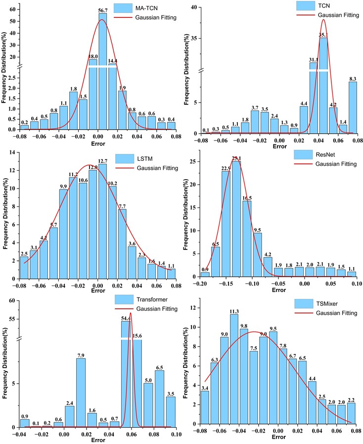
The MA-TCN model constructed in this paper effectively models dependency relationships under special data conditions compared to other networks. It derives feature data, dynamically adjusts fault period weighting in real-time based on physical rules, reduces the contribution of redundant channels, and accurately captures data failure timepoints. This enhances the model's feature learning capability and improves final prediction accuracy, achieving an value of 0.9629. Moreover, the error frequency distribution results in Fig. 9 indicate that the MA-TCN exhibits superior frequency distribution characteristics. This further validates the MA-TCN’s outstanding fitting performance in this prediction task.
7. Conclusions
This paper proposed and validated a novel MA-TCN model for diagnosing bearing faults in asynchronous motors, specifically addressing the challenges of low-frequency (1 Hz), low-dimensional, and unbalanced data common in industrial settings. The primary findings and their implications are as follows:
1) Efficacy of Proposed Attention Mechanisms: Ablation studies quantitatively confirmed the critical and synergistic contribution of the proposed multi-attention architecture. The baseline TCN model yielded an MAE of 0.1349, while the introduction of CA, SE, and TPA modules individually resulted in significantly improved MAE scores of 0.0348, 0.0412, and 0.0377, respectively. The final MA-TCN model, which integrates all three components, achieved the lowest MAE of 0.0244, demonstrating that these mechanisms work in concert to achieve the highest prediction accuracy.
2) Superior Performance Against Baselines: Following the validation of its internal components, the complete MA-TCN model demonstrated superior diagnostic performance in a comparative study against established baseline models, including LSTM, Transformer, and other. Specifically, our model’s top-tier results significantly surpassed the next-best baseline, quantitatively validating that our integrated architecture is more effective at capturing subtle fault signatures from sparse, low-dimensional, and unbalanced data streams.
3) Generalizability and Future Work: While this study focused on four specific, artificially induced fault types, the proposed model's architecture is fundamentally designed to learn underlying patterns from time-series data rather than memorizing specific fault signatures. Therefore, we hypothesize that the model possesses strong potential for generalization to other common bearing faults, since this potential is rooted in the distinct temporal patterns these faults produce in vibration and power data. Future work should validate this generalizability by testing the model on datasets from different motor models, a wider variety of fault types, and diverse operating environments. Investigating the model's performance under variable speed conditions and its potential for transfer learning to other rotating machinery also represent promising avenues for future research and further enhancing its practical engineering value.
References
-
J. Qiu et al., “Bearing fault diagnosis based on self-attention mechanism assisted classification generative adversarial network,” (in Chinese), Information and Control, Vol. 51, No. 6, pp. 753–762, Dec. 2022, https://doi.org/10.13976/j.cnki.xk.2022.2002
-
S. Tang, S. Yuan, and Y. Zhu, “Convolutional neural network in intelligent fault diagnosis toward rotatory machinery,” IEEE Access, Vol. 8, pp. 86510–86519, Jan. 2020, https://doi.org/10.1109/access.2020.2992692
-
R. Liu, B. Yang, E. Zio, and X. Chen, “Artificial intelligence for fault diagnosis of rotating machinery: A review,” Mechanical Systems and Signal Processing, Vol. 108, pp. 33–47, Aug. 2018, https://doi.org/10.1016/j.ymssp.2018.02.016
-
L. Hu et al., “Fault diagnosis of pumped storage unit bearings considering acoustic-vibration modal combination,” (in Chinese), Power System Protection and Control, Vol. 52, No. 11, pp. 1–10, Nov. 2024, https://doi.org/10.19783/j.cnki.pspc.231422
-
D. Shi and W. Wang, “Bearing fault feature extraction based on improved TVF-EMD and SVD,” (in Chinese), Machine Tool and Hydraulics, Vol. 52, No. 18, pp. 218–229, 2024.
-
Y. Gao and J. Zhang, “Bearing fault diagnosis based on EMD and FastICA,” (in Chinese), Journal of Mechanical Design and Manufacture, No. 6, pp. 48–52, Jun. 2024, https://doi.org/10.19356/j.cnki.1001-3997.2024.06.004
-
E. C. C. Lau and H. W. Ngan, “Detection of motor bearing outer raceway defect by wavelet packet transformed motor current signature analysis,” IEEE Transactions on Instrumentation and Measurement, Vol. 59, No. 10, pp. 2683–2690, Oct. 2010, https://doi.org/10.1109/tim.2010.2045927
-
L. Eren and M. J. Devaney, “Bearing damage detection via wavelet packet decomposition of the stator current,” IEEE Transactions on Instrumentation and Measurement, Vol. 53, No. 2, pp. 431–436, Apr. 2004, https://doi.org/10.1109/tim.2004.823323
-
M. Liu et al., “A review of bearing fault diagnosis in petrochemical machinery based on deep learning,” (in Chinese), Machine Tool and Hydraulics, Vol. 51, No. 6, pp. 171–180, 2023.
-
J. Sun, C. Yan, and J. Wen, “Intelligent bearing fault diagnosis method combining compressed data acquisition and deep learning,” IEEE Transactions on Instrumentation and Measurement, Vol. 67, No. 1, pp. 185–195, Jan. 2018, https://doi.org/10.1109/tim.2017.2759418
-
Z. Feng, M. Liang, and F. Chu, “Recent advances in time-frequency analysis methods for machinery fault diagnosis: A review with application examples,” Mechanical Systems and Signal Processing, Vol. 38, No. 1, pp. 165–205, Jul. 2013, https://doi.org/10.1016/j.ymssp.2013.01.017
-
Z. Wang et al., “Bearing fault diagnosis using multi-dilated convolutional network with adaptive feature selection,” (in Chinese), Information and Control, Vol. 53, No. 5, pp. 615–630, May 2024, https://doi.org/10.13976/j.cnki.xk.2024.3223
-
X. Jian and T. Zhang, “A novel lightweight bearing fault diagnosis model for imbalanced data,” (in Chinese), Control Engineering of China, Vol. 31, No. 4, pp. 729–737, Apr. 2024, https://doi.org/10.14107/j.cnki.kzgc.20211071
-
J. Liu, H. Wu, and H. Zhou, “Rolling bearing fault diagnosis method based on denoising multi-branch CNN and attention mechanism,” (in Chinese), Modular Machine Tool and Automatic Manufacturing Technique, No. 2, pp. 113–116, Feb. 2023, https://doi.org/10.13462/j.cnki.mmtamt.2023.02.026
-
D. Zhao, C. Tian, Z. Fu, Y. Zhong, J. Hou, and W. He, “Multi scale convolutional neural network combining BiLSTM and attention mechanism for bearing fault diagnosis under multiple working conditions,” Scientific Reports, Vol. 15, No. 1, p. 13035, Jan. 2025, https://doi.org/10.1038/s41598-025-96137-w
-
Y. Guo, J. Zhou, Z. Dong, H. She, and W. Xu, “Research on bearing fault diagnosis based on novel MRSVD-CWT and improved CNN-LSTM,” Measurement Science and Technology, Vol. 35, No. 9, p. 095003, Sep. 2024, https://doi.org/10.1088/1361-6501/ad4fb3
-
F. Liu et al., “Fault diagnosis of rolling bearings under varying speeds based on gray level co-occurrence matrix and DCCNN,” Measurement, Vol. 235, p. 114955, Aug. 2024, https://doi.org/10.1016/j.measurement.2024.114955
-
Q. Fan, Y. Liu, J. Yang, and D. Zhang, “Graph multi-scale permutation entropy for bearing fault diagnosis,” Sensors, Vol. 24, No. 1, p. 189, Nov. 2023, https://doi.org/10.2139/ssrn.4590574
-
S. Tian, D. Zhen, H. Li, G. Feng, H. Zhang, and F. Gu, “Adaptive resonance demodulation semantic-induced zero-shot compound fault diagnosis for railway bearings,” Measurement, Vol. 235, p. 115040, Aug. 2024, https://doi.org/10.1016/j.measurement.2024.115040
-
G. Li, M. Wei, D. Wu, Y. Cheng, J. Wu, and J. Yan, “Zero-sample fault diagnosis of rolling bearings via fault spectrum knowledge and autonomous contrastive learning,” Expert Systems with Applications, Vol. 275, p. 127080, May 2025, https://doi.org/10.1016/j.eswa.2025.127080
-
D. Mishra, P. C. Sahu, R. C. Prusty, and S. Panda, “A fuzzy adaptive fractional order-PID controller for frequency control of an islanded microgrid under stochastic wind/solar uncertainties,” International Journal of Ambient Energy, Vol. 43, No. 1, pp. 4602–4611, Dec. 2022, https://doi.org/10.1080/01430750.2021.1914163
-
C. Wang, J. Tian, F.-L. Zhang, Y.-T. Ai, Z. Wang, and R.-Z. Chen, “Simulation method and spectrum modulation characteristic analysis of typical fault signals of inter-shaft bearing,” Mechanical Systems and Signal Processing, Vol. 209, p. 111145, Mar. 2024, https://doi.org/10.1016/j.ymssp.2024.111145
-
X. Ma, Z. Li, J. Xiang, X. Sun, C. Chen, and F. Huang, “Nonlinear vibration analysis of rotor-bearing system with insufficient interference and bearing tilt,” International Journal of Mechanical Sciences, Vol. 287, p. 109966, Feb. 2025, https://doi.org/10.1016/j.ijmecsci.2025.109966
-
L. Zheng, Y. Xiang, and N. Luo, “Nonlinear dynamic modeling and vibration analysis for early fault evolution of rolling bearings,” Scientific Reports, Vol. 14, No. 1, p. 23687, Oct. 2024, https://doi.org/10.1038/s41598-024-75126-5
-
X. Huang, F. Cong, S. Xu, S. Dou, R. Yao, and N. Tang, “Asperity interaction induced vibration excitation of cylindrical roller bearings with localized defect,” Proceedings of the Institution of Mechanical Engineers, Part J: Journal of Engineering Tribology, Vol. 239, No. 5, pp. 632–648, Jan. 2025, https://doi.org/10.2139/ssrn.4458248
-
Y. Zou, X. Zhang, T. Liu, Y. Zhang, L. Li, and W. Zhao, “Rolling bearing fault diagnosis based on cross-attention fusion WDCNN and BiLSTM,” Computers, Materials and Continua, Vol. 83, No. 3, pp. 4699–4723, Jan. 2025, https://doi.org/10.32604/cmc.2025.062625
-
A. Mohanty, S. P. Parida, and R. R. Dash, “Modal response of sandwich plate having carbon-epoxy faceplate with different honeycomb core material and geometry considerations,” International Journal on Interactive Design and Manufacturing (IJIDeM), Vol. 18, No. 6, pp. 4223–4232, Jul. 2024, https://doi.org/10.1007/s12008-024-01975-z
-
Y. Si et al., “SCSA: Exploring the synergistic effects between spatial and channel attention,” Neurocomputing, Vol. 634, p. 129866, Jun. 2025, https://doi.org/10.1016/j.neucom.2025.129866
-
L. Lin, J. Wu, S. Fu, S. Zhang, C. Tong, and L. Zu, “Channel attention and temporal attention based temporal convolutional network: A dual attention framework for remaining useful life prediction of the aircraft engines,” Advanced Engineering Informatics, Vol. 60, p. 102372, 2024, https://doi.org/10.1016/j.aei.2024.102372
-
H. Yin, H. Xu, H. Zhang, J. Wang, and X. Fang, “MC-ABDS: A system for low SNR fault diagnosis in industrial production with intense overlapping and interference,” Applied Acoustics, Vol. 227, p. 110217, Jan. 2025, https://doi.org/10.1016/j.apacoust.2024.110217
-
G. E. P. Box, G. M. Jenkins, G. C. Reinsel, and G. M. Ljung, Time series analysis: forecasting and control. Hoboken, USA: John Wiley & Sons, 2015, p. 493.
-
J. Benesty, J. Chen, Y. Huang, and I. Cohen, “Pearson correlation coefficient,” in Noise Reduction in Speech Processing, 2455 Teller Road, Thousand Oaks California 91320 United States: Springer, 2009, pp. 1–4, https://doi.org/10.4135/9781412953948.n342
-
A. V. Oppenheim and R. W. Schafer, Discrete-Time Signal Processing. London, UK: Pearson Education, 2009.
-
S. Hochreiter and J. Schmidhuber, “Long short-term memory,” Neural Computation, Vol. 9, No. 8, pp. 1735–1780, Nov. 1997, https://doi.org/10.1162/neco.1997.9.8.1735
-
A. Vaswani et al., “Attention is all you need,” in Proceedings of the 31st International Conference on Neural Information Processing Systems, pp. 6000–6010, 2017, https://doi.org/10.65215/nxvz2v36
-
K. He, X. Zhang, S. Ren, and J. Sun, “Deep residual learning for image recognition,” in IEEE Conference on Computer Vision and Pattern Recognition (CVPR), pp. 770–778, 2016, https://doi.org/10.1109/cvpr.2016.90
-
Z. Chen et al., “TSMixer: An all-MLP architecture for time series forecasting,” Transactions on Machine Learning Research, 2023.
About this article

The authors have not disclosed any funding.
The datasets generated during and/or analyzed during the current study are available from the corresponding author on reasonable request.
Taohuang Liu: conceptualization, data curation, formal analysis, investigation, methodology, software, validation, visualization, writing-original draft preparation. Zhihua Hu: conceptualization, project administration, resources, funding acquisition, supervision. Gulizhati Hailati: visualization, validation, writing-review and editing. Lili Tao: data curation, software, writing-review and editing. Yiheng Hu: supervision, writing-review and editing. Feng Ding: supervision, writing-review and editing.
The authors declare that they have no conflict of interest.
