Small sample fault diagnosis method based on dual convolutional kernel feature fusion and channel attention weighted temporal convolutional network (DCK-CAM-TCN)

1. Introduction

The reliable operation of industrial equipment is of great significance for production efficiency and safety [1], and as a key component in mechanical equipment, the fault diagnosis of bearings is particularly important [2]. However, in actual industrial production, it is difficult to obtain fault data for many devices, and data collection becomes more complex and costly when faults occur less frequently [3]. This makes it difficult for the fault diagnosis system to train effectively and make accurate judgments when faced with limited fault data [4]. Therefore, how to achieve efficient and accurate fault diagnosis with small sample has become one of the key challenges in current research [5].

Traditional bearing fault diagnosis methods are largely based on techniques such as time-frequency analysis [6] and empirical mode decomposition [7]. These methods rely on manually designed features and are difficult to adapt to complex operating conditions and diverse signal patterns. With the development of deep learning technology, convolutional neural networks (CNNs) have gradually become a research hotspot due to their powerful feature extraction capabilities. Common neural network models, such as auto-encoders [8], deep belief networks (DBNs) [9], recurrent neural networks (RNNs) [10], deep convolutional neural networks (DCNNs) [11], and generative adversarial networks (GANs) [12], have made significant progress and have been applied in the field of fault diagnosis. The implementation of these methods typically requires designing novel and efficient network architectures or improving deep learning optimization algorithms. For example, Song et al. [13] proposed the Wide Convolutional Kernel Convolutional Neural Network (WKCNN) model to address the issue of low efficiency in traditional bearing fault diagnosis methods. Wang et al. [14] proposed a 1D-CNN based fault diagnosis method combining vibration and acoustic signals, achieving higher accuracy and robustness across various signal-to-noise ratios compared to single-modal approaches. Zhao et al. [15] put forward the CNN with mixed information model (MIXCN), which combines mixed information to enhance spatial feature extraction and reduce information loss in traditional convolution and residual connections, addressing the calculation efficiency limitations of existing complex convolutional neural networks.

In addition, small sample fault diagnosis has become a new research focus. For small sample fault diagnosis, researchers utilize feature extraction advantages of models or generate a large number of high-quality samples based on the distribution of real samples, or apply emerging machine learning techniques such as transfer learning. Lyu et al. [16] applied a novel data enhancement model gradient penalty separate classifier-Generative Adversarial Networks (GPSC-GAN), which addresses the challenge of generating high-quality multi-category fault samples by integrating a separate classifier and Wasserstein distance with gradient penalty. Li et al. [17] proposed a method based on two-dimensional vibration signal analysis and a Multi-Task Conditional Generative Adversarial Network (MTC-GAN), which effectively addresses the challenge of bearing fault diagnosis under small sample conditions through feature extraction and data augmentation, significantly improving diagnostic accuracy and robustness. Dong et al. [18] applied a fault diagnosis framework using dynamic models and transfer learning to address small sample problems, demonstrating improved fault identification through transferable features and reduced distribution discrepancies. Te et al. [19] developed a novel transfer learning framework for machinery fault diagnosis with sparse target data, utilizing paired source and target data to address distribution discrepancies and label mismatching, and demonstrate its superior performance over traditional methods through extensive experiments.

Although deep learning methods are widely used for efficient feature extraction in vibration signals, they lack the ability to dynamically adjust key feature channels. To address these issues, some researchers have introduced channel attention mechanisms into CNNs to enhance diagnostic performance through dynamic weighting. Huang et al. [20] proposed a CNN method with attention mechanisms that converts multivariate time series into images and incorporates prior knowledge, significantly improving fault diagnosis accuracy. Li et al. [21] proposed an attention mechanism-based improved CNN (AT-ICNN) to overcome the limitations of traditional diagnostic methods in extracting mechanical fault signals, enhancing fault feature extraction by combining CNN and hybrid attention mechanisms. Wang et al. [22] came up with a data-driven intelligent fault diagnosis method combining multi-head attention and CNN for automatic feature extraction and fault recognition of rolling bearings, achieving efficient bearing fault identification. Yang et al. [23] proposed a fault diagnosis method based on multi-layer Bidirectional Gated Recurrent Unit (BiGRU) and attention mechanism, combining CNN, GRU, and attention mechanism to improve the interpretability of neural networks in fault diagnosis.

Dual convolutional kernels extract multi-scale fault signatures by capturing features at different receptive fields, significantly improving the characterization and discernment of complex failure modes. In small sample fault diagnosis, large convolution kernels enhance robustness against noise-induced uncertainty [24], while deep small kernel stacks disentangle transferable fault representations from limited data. Li et al. [25] applied a dual-convolution kernel design, where parallel convolutional layers perform deep mining of fault features while the dynamic routing mechanism in capsule networks preserves spatial relationships among features, effectively addressing the challenges of small-sample dependency and poor generalization in rotating machinery fault diagnosis. Liu et al. [26] proposed a multi-scale kernel-based residual Convolutional Neural Network (CNN) for motor fault diagnosis, aiming to address the complexity of vibration signals under non-stationary conditions, by incorporating a multi-scale kernel algorithm to capture vibration patterns of different fault types. Chang et al. [27] introduced a Concurrent Convolutional Neural Network (C-CNN) method based on dual convolutional kernels, which extracts features using convolutional kernels of different scales to effectively address noise interference in wind turbine bearing fault diagnosis. Liao [28] presents a fault diagnosis method (RACNN) for AHUs in HVAC systems, combining rule-based detection and multi-kernel 1D CNNs for feature selection, achieving 99.15 % accuracy in offline tests. However, these methods are mostly based on CNN and do not fully utilize the dynamic characteristics of the time series.

In addition, time step information cannot be ignored in vibration signals. To effectively capture temporal features and hidden information at different positions in time series, a common strategy is to adopt gated Recurrent Neural Network (RNN) structures, such as Long Short-Term Memory (LSTM), or alternative architectures like Temporal Convolutional Networks (TCN). Although LSTM excels in temporal modeling, its large number of parameters makes it prone to overfitting in small-sample scenarios. Additionally, assuming that signals propagate information in only one direction is not reasonable. Therefore, TCN, as an alternative with fewer parameters and the ability to capture both forward and backward information, becomes a more optimal choice. Guo et al. [29] developed a fault diagnosis method for IGBT open-circuit faults in Modular Multilevel Converter (MMC) systems, combining TCN with Adaptive Chirp Mode Decomposition (ACMD) and Silhouette Coefficient (SC) to effectively extract long-term sequence features and maintain robustness under noisy conditions. Ai et al. [30] proposed an automatic temporal convolution network method based on TCN and enhanced elite genetic algorithm (SEGA) optimization for sensor faults of hypersonic aircraft, and combined SPRT and wavelet packet transform (WPT) to improve the accuracy of fault diagnosis. However, TCN lacks the ability to extract multi-scale features and focus key features, limiting further improvements in its diagnostic performance. Previous methods have achieved relatively satisfactory results, deep learning models typically require a large number of samples to achieve ideal generalization performance. However, due to the relatively small amount of annotated data, models often cannot fully learn various effective features from limited samples and are prone to overfitting, which increases the difficulty of learning [31]. In addition, the comparative study of new activation functions in small sample fault diagnosis has not been thoroughly explored.

Therefore, in response to the above issues, this paper proposes a small-sample fault diagnosis method based on dual convolutional kernel feature fusion and channel attention weighting within a Temporal Convolutional Network. By combining dual convolutional kernel feature fusion and a channel attention mechanism, the model not only extracts multi-scale features comprehensively but also adaptively focuses on key channel features. Under small sample conditions, the proposed method still demonstrates good diagnostic performance.

The main contributions of the paper are as follows:

1) Multi-Scale Feature Extraction via Dual Convolutional Kernel Fusion and Channel Attention Mechanism. This innovation overcomes the limitations of single-kernel feature extraction and significantly strengthens feature representation, offering a robust solution for small-sample fault diagnosis.

2) Temporal Convolutional Network (TCN) with Dilated Convolutions for Long-Range Dependency Modeling. This approach maintains computational efficiency while mitigating gradient vanishing issues. This innovation provides a stable and effective framework for temporal feature extraction under small-sample constraints.

3) Adaptive Pooling and End-to-End Classification Framework Integration. By combining adaptive average pooling with a fully connected classifier, this framework eliminates the need for manual feature engineering and reduces reliance on fixed-dimensional inputs. This innovation streamlines the diagnostic workflow and significantly enhances generalization performance and classification accuracy under limited data conditions.

The structure of this paper is as follows:

Chapter 2 elaborates on the fundamental theoretical principles of techniques such as Temporal Convolutional Networks and Channel Attention Mechanisms. Chapter 3 describes the overall framework of the proposed method in this paper. Chapter 4 introduces the sources, settings, and environment of the experimental data, evaluates the model performance through comparative experiments, and validates the effectiveness of the relevant mechanisms. Chapter 5 primarily summarizes the research findings.

2. Theoretical background

2.3. Temporal convolutional network (TCN)

The Temporal Convolutional Network (TCN) demonstrates outstanding performance in handling sequential data [33]. Its specific structure is shown in Fig. 1.

In its structure, causal convolutional layers strictly follow the principle of temporal causality. For the input sequence$\mathrm{ }x=[x_1,x_2,\cdots ,x_T]$, the output $y_t$ of causal convolution is calculated according to Eq. (10):

10

$y_t=\sum _{k=0}^{K-1} f\left(x_{t-k}\right),$

where $K$ is the size of the convolution kernel, and $f$ is the function corresponding to the convolution kernel. This structure effectively avoids the interference of future information on the current output, thereby accurately capturing the changing patterns in temporal data.

Dilated convolution expands the receptive field through the dilation factor $d$, for example, its output $y_t=\sum _{k=0}^{K-1} w_k{x}_{t-kd}$ (where $w_{ }$ is the dilated convolution kernel), successfully mining long-distance dependencies in the data without increasing computational complexity. The multi-layer stacking architecture of TCN enables each layer to gradually extract temporal features from local short-term to overall long-term.

The residual connection mechanism in the network (expressed as $y=F\left(x\right)+x$, where $F\left(x\right)$ is the convolutional transformation function) effectively alleviates the gradient problem that is prone to occur as the network depth increases.

During the training phase, stochastic gradient descent (SGD) is used in TCN for training [34]. The parameter update formula can be expressed as Eq. (11):

11

$\theta =\theta -\eta \frac{\partial L\left(\theta \right)}{\partial \theta },$

where $\eta$ represents the learning rate. Usually, the training process is optimized by combining the learning rate decay strategy, momentum method (where the update formula for velocity variable $v$ in momentum method is $v=\beta v-\eta \frac{\partial L\left(\theta \right)}{\partial \theta }$, and the parameter update formula is $\theta =\theta +v$, where $\beta$ is the momentum coefficient), and adaptive learning rate algorithms such as Adagrad, Adadelta, Adam, etc. At the same time, the use of regularization techniques to prevent overfitting ensures the generalization ability and reliability of TCN in temporal data processing applications.

Fig. 1Complete structure of TCN

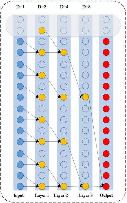
a) Dilated causal convolution

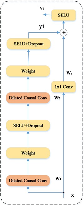
b) Hidden layer and residual connection

3. The proposed fault diagnosis method

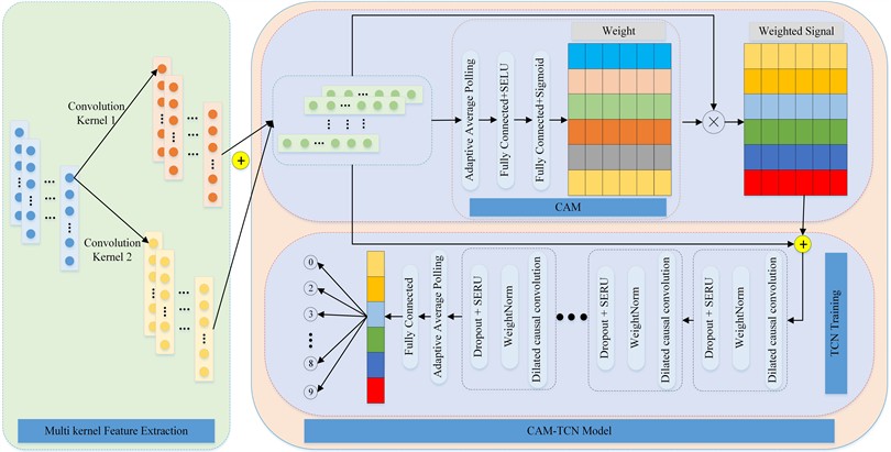
A small sample bearing fault diagnosis method based on dual convolutional kernel feature fusion and channel attention weighted temporal convolutional network is proposed, which combines feature fusion, attention mechanism, TCN and adaptive pooling. The specific steps of fault diagnosis based on DCK-CAM-TCN are as follows:

1) Data preprocessing: Convert the original one-dimensional signal into tensor format and normalize it to meet the input requirements of the model.

2) Multi scale convolution feature extraction: Extracting features from different frequency bands through two convolution branches, combined with pooling layers to reduce dimensionality.

3) Feature fusion and attention weighting: Multiply and fuse the element points at the corresponding positions extracted by two convolution kernels, and generate weighted features using attention mechanism.

4) Temporal Feature Modeling (TCN): Use Temporal Convolutional Network (TCN) to extract features with long-term dependencies and expand the receptive field through dilated convolution.

5) Reduce dimensions and classification decisions: After adaptive average pooling dimensionality reduction, it is mapped to the fault category space through a fully connected layer to complete classification.

The overall architecture of the DCK-CAM-TCN model is shown in Fig. 2.

Fig. 2Overall schema for the proposed network architecture of DCK-CAM-TCN

4. Experiment

4.2. Case 1: bearing fault data of West Reserve University

4.2.1. Dataset description

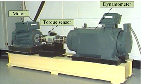
The driving end rolling bearing data provided by Case Western Reserve University is collected by the equipment shown in Fig. 3, wherein the faults (Inner ring fault (IR), Outer ring fault (OR) and Rolling element fault (RE)) are generated by electric discharge machining (EDM), the sampling frequency is 12 kHz, the load is 1HP, and the three damage degrees (the fault diameter is 0.118/0.356/0.533 mm respectively). An acceleration sensor located at the drive end of the motor housing collects acceleration data. Each fault type includes 102400 data points, of which 1024 data points are taken as samples, and each fault type has 100 samples. The specific fault types and labels are shown in Table 2.

Fig. 3CWRU test bench

4.2.2. Ablation comparative experiment

Vibration signals exhibit a nonlinear distribution, whereas neural networks inherently perform linear computations. To mitigate the issue of vanishing gradients, nonlinear non-saturating activation functions are commonly employed. To comprehensively evaluate the impact of activation functions on model performance, the nonlinear characteristics of these activation functions are first visualized in Fig. 4. Subsequently, the loss and accuracy curves under various activation functions, including ReLU, LeakyReLU, ELU, Softplus, and SELU, are systematically compared to assess their effectiveness in the proposed model.

Table 2Fault dataset description of CWRU

Fault type	Fault description	Label	Number of samples
Normal	Normal bearing	0	100
OR/RE/IR	0.1778 mm	1/2/3	100
OR/RE/IR	0.3556 mm	4/5/6	100
OR/RE/IR	0.5334 mm	7/8/9	100

All results are carried out under the CWRU dataset with a training-set ratio of 0.4, and the training loss and transfer accuracy are obtained, as shown in Fig. 5 and 6. It can be seen that all models can converge, with LeakyReLU having the maximum loss of 0.61. In terms of convergence stability, except for LeakyReLU, the other five activation functions are relatively stable, where the differences in loss are small in the later epochs. The difference in final losses among ReLU, Softplus, and SELU is about 0.005, while SELU requires fewer epochs and achieves the fastest convergence. Therefore, in the subsequent experiments, SELU is used as the activation function.

This section aims to evaluate the performance differences among Adam, Adagrad, and Adadelta optimizers in deep learning tasks, with a focus on convergence speed, model accuracy, and training stability. The rationale for selecting Adam as the primary optimizer is validated through systematic comparisons. The study employs CWRU datasets and measures key metrics including training loss, test accuracy, and gradient noise sensitivity. The results are summarized in Table 3, highlighting the performance of each optimizer under identical hyperparameter settings.

Fig. 4Different activation functions

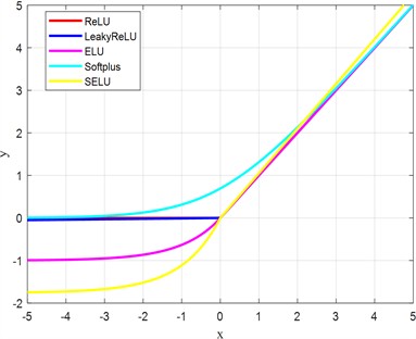
Fig. 5Loss under different activation functions

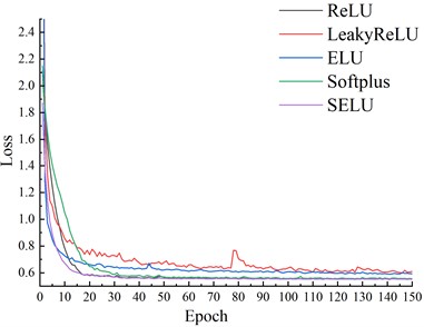
Fig. 6Accuracy under different activation functions

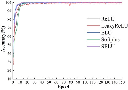
Table 3Test results of different optimizers

Optimizer	Test accuracy (%)	Convergence epochs	Final training loss
Adam	100	25	0.52
Adagrad	94.86	33	0.75
Adadelta	92.54	30	1.10

The ablation study confirms that Adam outperforms Adagrad and Adadelta in most critical metrics. Its adaptive learning rate mechanism, combined with momentum-based updates, provides superior convergence speed and stability, making it suitable for complex, high-dimensional tasks. While Adagrad remains effective for sparse data, its learning rate decay limits long-term training. Therefore, Adam is selected as the default optimizer in this study due to its robustness and efficiency.

This section introduces a systematic evaluation of the learning rate (LR) impact on model performance. The goal is identify the optimal LR range for the model and highlight the trade-offs between training efficiency and final performance. The results are summarized in Table 4, with all other hyperparameters fixed.

The learning rate sensitivity analysis confirms that 0.001 is the optimal LR for this model, achieving the highest test accuracy and lowest training loss while maintaining rapid convergence and stability.

Table 4Experimental results of different learning rates

Learning rate	Test accuracy (%)	Final training loss	Convergence speed (epochs)
0.0001	97.50	1.05	54
0.0005	98.83	0.61	53
0.001	100	0.52	25
0.005	97.83	0.62	48
0.01	98.50	0.63	53

Fig. 7Accuracy values of test-set under different model and training-set ratio

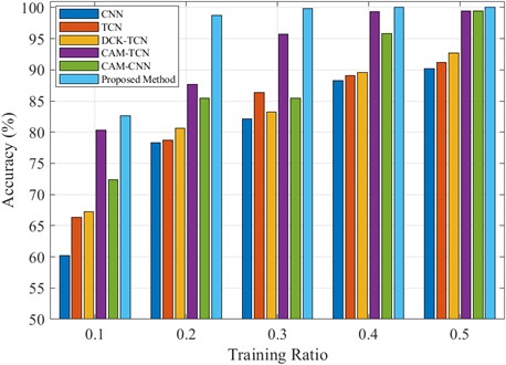
To verify the diagnostic performance of the model in small samples, compares the diagnostic accuracy of the test set under different training set ratios in this paper. Fig. 7 illustrates the highest accuracy achieved upon model convergence. The experimental results demonstrate that the traditional CNN and TCN performs the worst under small sample conditions. As the proportion of the training set increases, the accuracy of CNN and TCN gradually improves, reaching 90.17 % and 91.23 % respectively, when 50 % of the training samples are used. However, they still lag behind the other models presented in this study. Comparative analysis between TCN and DCK-TCN demonstrates that the DCK module significantly enhances the model's classification accuracy. The CAM-TCN and CAM-CNN models significantly enhance feature extraction by incorporating a Channelized Attention Mechanism (CAM), with a particularly notable improvement under small sample conditions. CAM-TCN achieves accuracies of 80.36 % and 87.67 % at 10 % and 20 % of the training set, respectively, outperforming CAM-CNN, which reaches 72.34 % and 85.46 %. This suggests that the time series modeling capability of CAM-TCN better facilitates fault identification in small sample scenarios. The proposed method consistently outperforms the other models, achieving an accuracy of 82.67 % across all training set proportions, and reaching 100 % test accuracy at 40 % of the training set. These results demonstrate better diagnostic performance in small sample tests.

4.2.3. Visual analysis of results

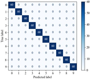
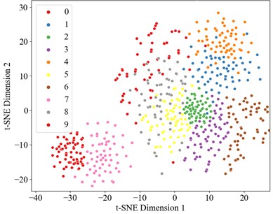
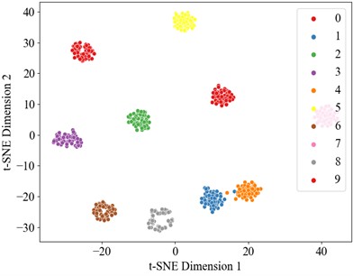
Optimal performance is achieved with 100 % accuracy when utilizing the full 40 % training dataset, establishing this as a benchmark for comparative analysis. Therefore, the dataset was divided into a training set and test set in a 4:6 ratio, with the experimental results presented below. Fig. 8 and 9 illustrate the accuracy curve and the loss curve, respectively. The accuracy curve basically converges after 25 epochs. To better evaluate the contribution of each module in fault diagnosis, this study applies visual dimension reduction on the raw data, feature fusion data, CAM data, and data processed by the TCN sequentially through t-SNE analysis, as shown in Fig. 10. The results reveal that the data distribution becomes more concentrated after each processing layer, with the distinction between categories significantly enhanced. Notably, the diagnostic performance between fault categories is greatly improved, particularly in the data weighted by channel attention. The TCN module further optimizes feature representation, leading to a substantial improvement in fault classification performance. The confusion matrix results for the test set (Fig. 11) demonstrate that the collaboration of the modules effectively enhances the model’s ability to identify small sample fault diagnosis tasks, confirming the effectiveness of the proposed method in fault diagnosis.

Fig. 8Accuracy curve

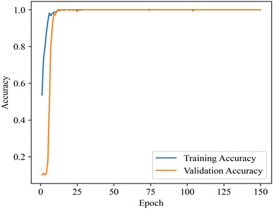
Fig. 9Loss curve

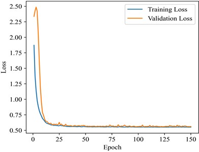
Fig. 10t-SNE visualization

a) Original data T-SNE

b) t-SNE after convolution fusion

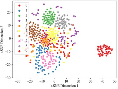
c) t-SNE after attention mechanism

d) t-SNE after TCN

Fig. 11Confusion matrix diagram

4.3. Case 2: Fault data of mechanical fault comprehensive test bench

To validate the generalization ability of the proposed method, this study further conducted experimental verification using the fault data from the mechanical fault comprehensive test bench.

4.3.1. Dataset description

The mechanical failure comprehensive test stand from SQ Company (USA) is employed to simulate bearing failure data at the load end. The Mechanical Fault Comprehensive Test Bench is illustrated in Fig. 12. The bearings at the load end is ER-12K. A 0.5 mm deep groove is machined on the outer and inner rings, as well as the rolling elements, to simulate failure of the bearing outer, inner rings and rolling elements fault, respectively. The motor operates at speeds of 1200 rpm, 1800 rpm, and 2400 rpm, with a sampling frequency of 12,800 Hz. The vibration signals utilized in this study are acquired by an acceleration sensor located at the load end. Each fault type consists of 102,400 data points, from which 1,024 data points are selected as samples, with each fault type containing 100 samples (training set: test set = 4:6). The corresponding labels for the various data types are presented in Table 5.

Fig. 12Mechanical fault comprehensive test bench

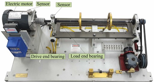
Table 5Dataset description of comprehensive test bench

Fault type	Rotational speed	Label	Number of samples
Normal	1200 r/min	0	100
RE /IR/OR		1/2/3	100
RE /IR/OR	1800 r/min	4/5/6	100
RE /IR/OR	2400 r/min	7/8/9	100

4.3.2. Result and analysis

This experiment compares the performance of four models in classifying a dataset with a training-to-test set ratio of 4:6, with the results presented in Fig. 13. Fig. 13 illustrates the highest accuracy achieved upon model convergence. The traditional CNN achieved an accuracy of 88.14 %, demonstrating its ability to handle basic tasks, though it does not fully capture the deep correlations within the feature data. The DCK module improves the model's classification accuracy, as shown by comparing TCN and DCK-TCN. In contrast, the model combining CAM-TCN significantly improved performance, attaining an accuracy of 96.78 %. This indicates that the attention mechanism enhances the model's ability to process temporal data. Further optimization of the CNN model by integrating the attention mechanism (CAM-CNN) resulted in an accuracy of 98.83 %, highlighting its superior capability in feature extraction and the distribution of importance weights. Finally, the DCK-CAM-TCN model achieved perfect accuracy of 99.98 %, demonstrating that this combination effectively captures data features and addresses the classification challenges in the experiment.

These results suggest that the introduction of model complexity and specific mechanisms, such as CAM and DCK, significantly enhances classification performance. The loss curve shown in Fig. 14 indicates that the loss steadily decreases and stabilizes as training progresses, signifying the successful convergence of the model. Additionally, the accuracy curve in Fig. 15 illustrates the continuous improvement in both training and validation accuracy, ultimately reaching 100 % accuracy.

Fig. 13Accuracy values of test-set under different mode

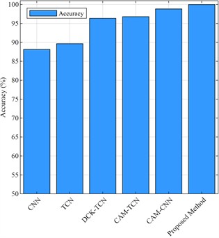
Fig. 14Accuracy curve

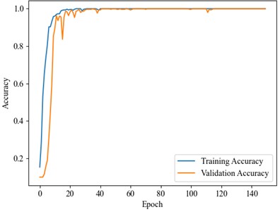
Fig. 15Loss curve

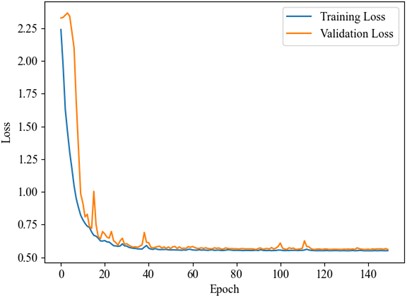
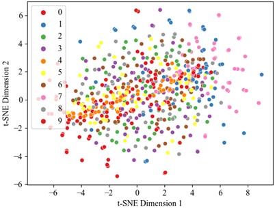
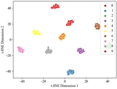
Fig. 16t-SNE visualization

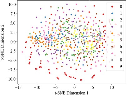
a) Original data T-SNE

b) t-SNE after convolution fusion

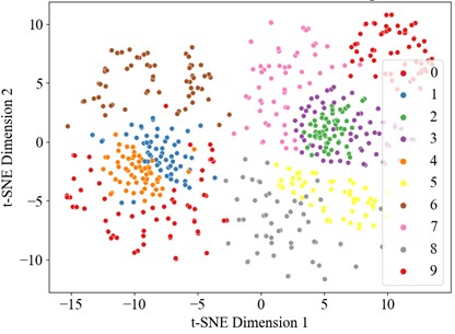
c) t-SNE after attention mechanism

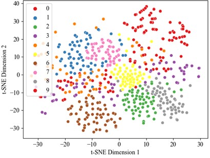
d) t-SNE after TCN

4.3.3. Visual analysis of results

The dataset also was divided into a training set and test set in a 6:4 ratio, with the experimental results presented in the Fig. below. The t-SNE dimensionality reduction visualization results are shown in Fig. 16, where the learning effects of each layer's features can be intuitively observed. In the DCK-CAM-TCN model, the t-SNE plots for each module clearly demonstrate the separation between categories, proving that the introduction of the CAM and DCK mechanisms effectively enhances the model’s ability to process data features. Particularly in the deeper feature mappings of the model, the data distribution becomes more concentrated, and the differences between categories become more pronounced, further validating the effectiveness of the model. Overall, with the increase in model complexity and the introduction of these mechanisms, the DCK-CAM-TCN demonstrates exceptional performance and superior generalization ability in fault diagnosis.

5. Conclusions

This paper presents a novel small-sample fault diagnosis method based on dual convolutional kernel feature fusion and channel attention weighted temporal convolutional network (DCK-CAM-TCN) to address the challenges of insufficient labeled data and low accuracy in fault diagnosis of industrial equipment. Dual convolutional kernel feature fusion enables the extraction of both low-frequency and high-frequency features, providing comprehensive multi-scale information. The channel attention mechanism adaptively weights the channels to focus on crucial features, enhancing the model's discriminative ability. Temporal Convolutional Network (TCN) is employed to handle long-sequence data effectively, capturing long-term dependencies and expanding the receptive field.

Experimental results on two datasets demonstrate the superiority of the proposed method. It shows that the data distribution becomes more concentrated and the category distinctions are enhanced after each processing step, indicating that the model can extract more discriminative features. In comparison with traditional Convolutional Neural Networks (CNNs) and other models, DCK-CAM-TCN achieves significantly higher accuracies, especially in small-sample scenarios. For instance, with only 20 % of the training data, it reaches 97 % convergence accuracy on the test set in certain cases, highlighting its excellent diagnostic capabilities. Performance peaks at 100 % accuracy when 40 % of the training data is used. Visual analysis through t-SNE further validates the effectiveness of each module in the model.

In summary, the DCK-CAM-TCN model proposed in this paper provides an effective solution for small-sample fault diagnosis. However, the model’s generalization capability in extreme small-sample regimes below 10 % training data requires further exploration. Future research could focus on further optimizing the model, exploring its application in more complex industrial scenarios, and potentially combining it with other emerging techniques to achieve even better performance in the field of fault diagnosis.