A feature lightweight image coding method for fault diagnosis of hydraulic motor bearings: PVIE

Teng, Xiaomin; Xing, Huiying; Wang, Wansheng; Li, Jing; Ma, Yunlin

doi:10.21595/jve.2026.25992

Journal of Vibroengineering

Browse Journal

Submit article

Published: June 4, 2026

Check for updates

A feature lightweight image coding method for fault diagnosis of hydraulic motor bearings: PVIE

Xiaomin Teng¹

Huiying Xing²

Wansheng Wang³

Jing Li⁴

Yunlin Ma⁵

^{1, 4}Department of Hydraulic Engineering, Shandong Water Conservancy Vocational College, Rizhao, China

²River and Lake Protection and Construction Operation Safety Center of Haihe River Water Conservancy Commission, MWR, Tianjing, China

^{3, 5}College of Water Conservancy and Hydropower Engineering, Hohai University, Nanjing 210098, China

Corresponding Author:

Wansheng Wang

Cite the article Download PDF

Article in Press

Downloads 0

Abstract

To address the critical challenge of low diagnostic accuracy in multistate bearing fault diagnosis caused by inefficient discriminative feature extraction under varying operating conditions, this paper proposes a novel Parameter-weighted Viridis Image Encoding (PVIE) method. Unlike conventional image encoding techniques (e.g., GADF, GASF, MTF, RP) that often suffer from high computational complexity and limited feature separability in complex scenarios, PVIE integrates Variational Mode Decomposition (VMD) with a newly designed Parameter-weighted Euler Difference Feature Extraction (PWEDFE) module. This module explicitly enhances the nonlinearity and periodicity of fault signatures, mapping them into lightweight 2D feature images via Viridis Feature Value Mapping (VFVM). Extensive experiments on two benchmark datasets demonstrate that PVIE achieves exceptional diagnostic accuracies of 99.92 % and 99.74 %, respectively. Compared to state-of-the-art encoding methods, PVIE improves average accuracy by 21.06 % to 39.78 % while reducing diagnostic time by 53.3 %, significantly outperforming existing approaches in both accuracy and efficiency. Furthermore, the method exhibits robust performance under strong noise interference and small-sample scenarios. These results confirm that PVIE offers a substantial advancement over current research by providing a more discriminative, lightweight, and robust solution for real-time industrial fault diagnosis.

A feature lightweight image coding method for fault diagnosis of hydraulic motor bearings: PVIE

Highlights

A lightweight PVIE method is proposed for multi-condition bearing fault diagnosis.
PWEDFE enhances nonlinear and periodic fault features from VMD-decomposed signals.
VFVM converts enhanced features into compact Viridis-based 2D feature images.
PVIE achieves 99.92 % and 99.74 % accuracies on two benchmark datasets.
The method maintains strong robustness under noise interference and small samples.

1. Introduction

In modern power systems, pumped hydro storage (PHS) serves as a flexible, efficient, and clean regulating power source and plays a critical role in ensuring the safe and stable operation of the grid. The motor bearings in PHS units often operate under harsh conditions, and their reliability is of paramount importance to the overall security of new-type power systems. As key components in rotating machinery, rolling bearings directly influence the performance and reliability of mechanical systems [1, 2]. Statistics show that more than 30 % of failures in rotating machinery are attributable to bearing degradation [3], particularly under high-load, high-speed, and continuous high-intensity operating conditions, which render bearings susceptible to early-stage damage.

Vibration signals from bearings contain rich information related to incipient faults; thus, effective monitoring of these signals is essential for early fault detection and prevention of catastrophic failures. With the advancement of industrial automation and digitalization, the volume of bearing vibration data has grown exponentially. However, conventional fault diagnosis methods struggle to extract discriminative features from massive, high-dimensional, and non-stationary vibration signals, leading to limited accuracy and robustness in diagnostic models. Consequently, there is an urgent need for novel approaches capable of efficiently processing large-scale vibration data and achieving high-precision fault diagnosis.

A typical bearing fault diagnosis framework comprises three core stages: vibration signal acquisition, fault feature extraction, and fault pattern recognition [4, 5]. Among these, the effectiveness of feature extraction fundamentally determines the accuracy of subsequent classification and is therefore a prerequisite for precise diagnosis [6]. Nevertheless, the operational conditions of bearings – such as load and rotational speed – are highly variable in practice, which introduces significant challenges in stably extracting fault-relevant features and consequently compromises the generalization and reliability of diagnostic models [7].

In recent years, numerous signal processing and feature extraction techniques have been applied to bearing fault diagnosis. For instance, Li et al. [8] employed VMD to decompose raw vibration signals into a set of Intrinsic Mode Functions (IMFs), discarded low-amplitude IMFs, and then performed envelope power spectrum analysis on the retained components to identify compound faults. Jin et al. [9] optimized VMD parameters using an improved Grey Wolf Optimizer (GWO) to directly extract fault features from raw signals. He et al. [10] integrated Particle Swarm Optimization (PSO) with VMD for adaptive parameter tuning, followed by a component selection strategy to enhance fault signatures. Lei et al. [11] proposed a composite index 𝑃 to screen and reconstruct IMFs obtained via Empirical Mode Decomposition (EMD), thereby amplifying fault-related information prior to envelope spectrum analysis. Cong et al. [12] utilized kurtosis-based criteria to select dominant IMFs from EMD outputs, effectively suppressing noise interference. Zhao et al. [13] combined VMD with the Hilbert transform to construct Hilbert envelope spectra, which were then formatted into feature matrices and fed into a Deep Belief Network (DBN) for fault classification. Shao et al. [14] developed a Modified Stacked Autoencoder (MSAE) based on an adaptive Morlet wavelet, enabling automatic diagnosis of multiple fault types and severity levels by establishing a nonlinear mapping between raw non-stationary vibration data and fault states. Zhang et al. [15] proposed an enhanced non-convex sparse decomposition method using an improved Morlet Continuous Wavelet Transform (CWT), where a waveform-adjustment factor was introduced to construct a tunable Morlet wavelet basis capable of matching diverse fault-induced impulse waveforms. Pan et al. [16] fused Fast Fourier Transform (FFT) and CWT to extract multi-domain features from raw vibration signals, demonstrating high classification accuracy and robustness in experimental validation.

Despite their success under specific conditions, these methods often exhibit limited performance in complex scenarios involving multiple operating conditions, numerous fault types, and subtle inter-condition differences, where discriminative feature extraction remains challenging.

Convolutional Neural Networks (CNNs), as representative deep learning models, have demonstrated exceptional capability in feature learning and classification, particularly in image recognition tasks [17, 18]. To leverage the powerful image-based feature extraction capacity of CNNs, researchers have transformed one-dimensional vibration signals into two-dimensional images for network input. For example, Bian et al. [19] reconstructed vibration sequences into 2D grayscale matrices via fixed-interval sampling and fed them into a deep residual shrinkage network. Wang et al. [20] adopted transfer learning with image-encoded vibration data to achieve high-accuracy fault diagnosis. While grayscale image encoding offers advantages in terms of low data volume and fast training, it generally exhibits poor noise resilience. Alternatively, advanced image encoding techniques – such as Gramian Angular Difference Fields (GADF) [21, 22], Markov Transition Fields (MTF) [23, 24], and Recurrence Plots (RP) [25, 26] have been widely employed. These methods preserve temporal dynamics and nonlinear characteristics of signals, offering enhanced noise robustness and diagnostic accuracy. However, they typically generate high-dimensional, large-volume images, significantly increasing computational overhead and inference latency, thereby hindering their applicability in industrial settings that demand real-time performance and lightweight solutions.

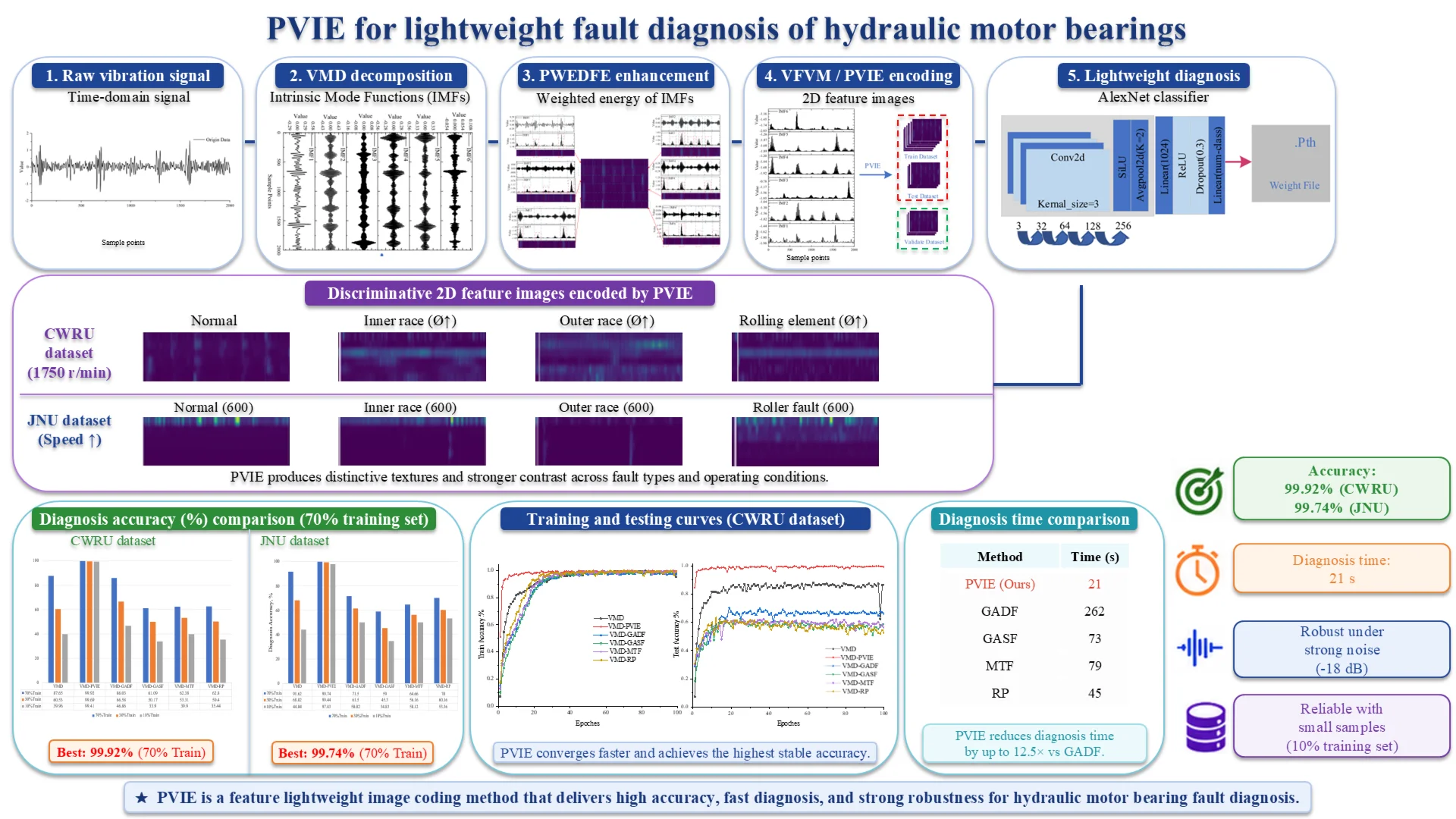
To address these issues, this paper proposes a lightweight image coding method, namely Parameter-weighted Viridis Image Encoding (PVIE), which effectively converts multi-condition bearing fault data into discriminative two-dimensional feature images. These images are then processed by the lightweight CNN architecture AlexNet to achieve accurate fault diagnosis under different operating conditions. The overall process of the proposed method is shown in Fig. 1.

The main contributions of this work are as follows:

Adaptive signal decomposition is carried out through VMD, and then discriminative features are extracted from a single IMF using weighted Euler differential feature representation, thereby enhancing the separability of fault modes under different operating conditions.

Fig. 1Overall flow chart of this paper

2. Proposed method

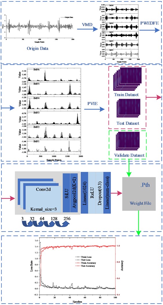
To address the limitations of existing methods in multi-condition bearing fault diagnosis, such as poor discriminative feature extraction leading to low diagnostic accuracy and low diagnostic efficiency in image-based fault diagnosis, this paper proposes a multi-condition bearing fault image conversion method that combines VMD, parameter-weighted Euler difference feature extraction, and Viridis feature value mapping. After converting the bearing fault data using PVIE, a simple neural network structure, AlexNet, is used for fault diagnosis. Since the focus of this article is not on the network structure, we do not provide a detailed description of AlexNet; instead, we only describe the parameters used in the network. The training configuration of the model is as follows: the optimizer is Stochastic Gradient Descent (SGD), the initial learning rate is set to 0.001, the momentum factor is 0.9, and the weight decay coefficient is 0.0005. The batch size is set to 64, and the number of training epochs is 100. During the training process, the learning rate adopts an exponential decay strategy, decaying once every 20 epochs with a decay coefficient of 0.9. All experiments are conducted under the same hardware environment and with the above unified hyperparameters to ensure the comparability and reproducibility of the results.

2.1. Variational mode decomposition

The VMD algorithm is an adaptive non-recursive modal decomposition method. This method utilizes the alternating direction method of multipliers algorithm to iteratively solve the constrained variational model, thereby obtaining the optimal solution for K IMFs with center frequencies $ω_{k}$ . The decomposition process of VMD can be summarized as follows:

Step 1: Initialization $\{μ_{k}^{1}\}$ , $\{ω_{k}^{1}\}$ , $λ^{1}$ , $n \leftarrow 0$ .

Step 2: Let $n = n + 1$ , $k = k + 1$ , update ${\hat{μ}}_{k}^{n + 1}$ and $ω_{k}^{n + 1}$ separately using Eq. (1) and Eq. (2). Stop iteration when $k = K$ :

1

{\hat{μ}}_{k}^{n + 1} (ω) = \frac{\hat{f} (ω) - \sum_{i \neq k} {\hat{μ}}_{i}^{n + 1} (ω) + \frac{\hat{λ} (ω)}{2}}{1 + 2 α (ω - ω_{k})} .

Step 3: Update ${\hat{λ}}^{n + 1}$ using the above equation:

2

{\hat{λ}}^{n + 1} (ω) = {\hat{λ}}^{n} (ω) + τ (\hat{f} (ω) - \sum_{k} {\hat{μ}}_{k}^{n + 1} (ω)) .

Step 4: Given $ε$ > 0, stop iteration when Eq. (3) is satisfied. Otherwise, repeat steps 2 to 4:

3

ε > \sum_{k} \frac{{‖{\hat{μ}}_{k}^{n + 1} - {\hat{μ}}_{k}^{n}‖}_{2}^{2}}{{‖{\hat{μ}}_{k}^{n}‖}_{2}^{2}} .

The parameters $K$ and $α$ in the equation are preset parameters.

2.2. PV image encoding

PVIE highlights subtle features in bearing fault signals, enhancing the importance of discriminative features, and then generates two-dimensional images of fault features through heatmap mapping.

2.2.1. Parameter weighted Euler difference feature extraction

In multi-condition bearing fault diagnosis, due to the low discriminability of fault features under different conditions, conventional feature extraction methods struggle to effectively extract discriminative features, leading to difficulty in accurate diagnosis of bearing faults under multi-conditions. Therefore, this paper proposes a feature extraction method based on a modified Euler formula, aiming to differentiate fault features under different conditions and highlight discriminative features.

This method involves multiple mathematical transformation steps, combining data scaling, trigonometric function transformation, and exponential transformation to effectively extract complex latent features. First, data is standardized to the [0, 1] interval to eliminate dimensional effects and provide a consistent scale for subsequent transformations. Next, the normalized data is converted into angle values using the arccosine function, introducing periodic and nonlinear information. Then, trigonometric and exponential functions are applied to further transform the data, generating feature values with higher nonlinearity to highlight meaningful feature differences. This comprehensive approach not only enhances the capture of spatial signal features but also improves data feature expression, laying a solid foundation for further analysis and modeling.

The specific steps of PWEDFE are as follows.

Step 1: Data Scaling.

To ensure that different features share the same scale and to eliminate dimensional effects between the data, the original data is first standardized. Let the original data be represented as $x x$ . The normalization formula is:

4

x_{i} = \frac{x - \min (x)}{\max (x) - \min (x)},

where, $x_{i}$ denotes the standardized data value, while $\min (x)$ and $\max (x)$ represent the minimum and maximum values in the data column, respectively. This formula linearly scales the data to the [0, 1] range, ensuring that all data points are within a uniform scale.

Step 2: Calculation of the Arccosine Value.

After completing the standardization, the next step is to calculate the arccosine values of the standardized data to obtain the corresponding angles. This process can be expressed as:

5

ϕ = \arccos (x_{i}) .

In this case, $ϕ$ is the arccosine angle corresponding to the standardized data $x_{i}$ . The $a r c c o s$ function maps the standardized data to angles in the range [0, $π$ ]. This step introduces a nonlinear transformation that effectively captures the periodic characteristics of the data.

Step 3: Feature Calculation.

Based on the transformation by Euler formula, this paper defines two new features that incorporate the nonlinear effects of trigonometric and exponential functions:

6

F i e s t E u l e r = \cos (ϕ) + x_{i} \sin (ϕ),

7

S e c o n d E u l e r = \exp (x_{i} ϕ) .

FirstEuler combines the cosine of angle $ϕ$ , denoted as $\cos (ϕ)$ , with the product of normalized data $x_{i}$ and the sine of angle $\sin (ϕ)$ . This combination of trigonometric functions captures both the periodicity and nonlinear patterns in the data. SecondEuler applies a nonlinear expansion to the product of normalized data $x_{i}$ and angle $ϕ$ using an exponential function.

Step 4: Weighted Values:

8

M_{1} = M e a n (F i r s t E u l e r),

9

M_{2} = M e a n (S e c o n d E u l e r),

Step 5: PWEDFE:

10

P W E D F E = M_{1} • F i r s t E u l e r - M_{2} • S e c o n d E u l e r .

The above method employs standardization, angle calculations, nonlinear transformations, and feature differentiation to form two feature extraction methods: FirstEuler and SecondEuler. By performing a differential operation on these two features, this technique extracts the discriminative features from the data, combining the nonlinear effects of trigonometric and exponential transformations. This approach provides a new perspective on feature extraction, enhancing the expressive capability of the data for subsequent analysis and model training.

2.2.2. Viridis feature value mapping: VFVM

VFVM is a color mapping scheme used for numerical data visualization. It represents different values through color changes, thus making the data easier to understand and interpret. The notable feature of Viridis color mapping is that it maps the initial value to deep purple, transitions the intermediate value to bright yellow, and finally uses bright yellow to represent the larger value. First, standardize the data to between 0 and 1, where 0 represents the minimum value and 1 represents the maximum value. Then, the standardized values are associated with specific color values. In Viridis, colors are represented by three values: red (R), green (G), and blue (B), and the value range of each color component is from 0 to 255. Finally, the corresponding color value is calculated through interpolation. The specific interpolation method is as follows:

11

R (x) = R_{0} + (R_{1} - R_{0}) • \frac{x - x_{0}}{x_{1} - x_{0}},

12

G (x) = G_{0} + (G_{1} - G_{0}) • \frac{x - x_{0}}{x_{1} - x_{0}},

13

B (x) = B_{0} + (B_{1} - B_{0}) • \frac{x - x_{0}}{x_{1} - x_{0}},

where, $(R_{0}, G_{0}, B_{0})$ and $(R_{1}, G_{1}, B_{1})$ are the RGB values corresponding to input values $x_{0}$ and $x_{1}$ .By following these steps, we can map any value between 0 and 1 to the corresponding color by VFVM. In conclusion, the original bearing fault signal is converted into a two-dimensional image using VFVM, forming the fault dataset.

Although PVIE and methods like GADF generate $N$ × $N$ images in the same way, there are fundamental differences in the computational complexity of their encoding processes. The core operations of GADF and similar methods involve Gram matrix calculations, state transition probability statistics, or distance matrix calculations. These operations involve a large number of addition and multiplication operations or conditional judgments, and the calculation of each element depends on multiple other elements. However, the VFVM mapping in PVIE is independent linear interpolation pixel by pixel, and the calculation of each pixel only depends on the corresponding position's PWEDFE eigenvalue, without the need for cross-pixel calculations. Therefore, although both have a progressive complexity of O( $N^{2}$ ), the actual constant factor of PVIE’s operation is much smaller than that of the comparison methods.

3. Bearing fault dataset

To verify the generalization of the proposed method, this paper adopts two different bearing fault datasets for verification. The most significant difference between the two datasets lies in the different bearing models used. By verifying the diagnostic performance of the diagnostic method for the fault data generated by different bearing models, the generalization performance of the diagnostic method is verified.

3.1. Case Western Reserve University bearing dataset (CWRU)

The bearing fault experimental setup at Case Western Reserve University primarily consists of three components: an induction motor, a torque transducer, and a dynamometer. Intelligent sensors are installed at both the drive end and the fan end of the bearings to collect vibration signals. The drive end employs SKF6205 single-row deep groove ball bearings, while the fan end utilizes SKF6203 single-row deep groove ball bearings. Faults on these bearings are introduced through electro-discharge machining. The specific fault types are detailed in Table 1.

Table 1CWRU bearing data

Bearing speed	Load / hp	Fault type	Fault diameter / mm
1750 r/min	1	Normal	–
		Inner race	0.1778/0.3556/0.5334
		Outer race	0.1778/0.3556/0.5334
		Rolling	0.1778/0.3556/0.5334
1772 r/min	2	Normal	–
		Inner race	0.1778/0.3556/0.5334
		Outer race	0.1778/0.3556/0.5334
		Rolling	0.1778/0.3556/0.5334
1797 r/min	3	Normal	–
		Inner race	0.1778/0.3556/0.5334
		Outer race	0.1778/0.3556/0.5334
		Rolling	0.1778/0.3556/0.5334

To evaluate the proposed method’s capability to overcome variations in rotational speed, this study selects data from three distinct speeds. For each speed, the bearing data encompasses both normal conditions and three types of faults. Each fault type is further categorized into three subclasses based on fault diameter, resulting in a total of 30 fault conditions for multi-condition fault diagnosis experiments.

3.2. Jiangnan University bearing fault dataset (JN)

The Jiangnan University (JNU) bearing fault dataset is derived from the fault diagnosis test bench of the rolling bearing centrifugal fan system at Jiangnan University, and is mainly used for research on fault diagnosis and health status identification of rolling bearings. As shown in Table 2, two types of rolling bearings were used in the tests, with specific bearing models corresponding to different health conditions. Among them, N205 bearings were used to simulate normal conditions, outer race fault conditions, and roller fault conditions, while NU205 bearings adopted a separable outer race design and were specifically used to simulate inner race fault conditions. A single-sensor arrangement was employed for vibration signal acquisition, with the following specific parameters: the acquisition equipment was a PCBMA352A60 accelerometer, which measured vertical vibration signals, the sampling frequency was set to 50 kHz, and the sampling duration for each working condition was 20 seconds. The dataset contains combined samples of 4 health states and 3 operating conditions. The health state categories include Normal, Inner Race Fault, Outer Race Fault, and Roller Fault. The operating condition parameters are distinguished by rotational speed, which are 600 rpm, 800 rpm, and 1000 rpm respectively; the sample characteristic is that it covers 4 health states under the same rotational speed, which provides complete data support for intelligent diagnosis and fault identification under specific operating conditions.

Table 2JNU bearing data

Contents	N205 (mm)	NU205 (mm)
Outer diameter of bearing 1	52	52
Outer diameter of bearing 2	25	25
Width of bearing	15	15
Roller diameter	7	7
Number of rollers	10	11
Contact angle	0 rad	0 rad
Outer race defect (width × depth)	0.3×0.25 mm
Roller defect (width × depth)	0.3×0.25 mm
Inner race defect (width × depth)	–	0.3×0.25 mm

3.3. Generation of fault datasets

For the conversion processing of multi-condition bearing fault data, VMD was first adopted to perform modal decomposition on the original fault data. The decomposed feature data are converted into feature images via PVIE, which are then used as input samples for the diagnostic model. The specific conversion process is illustrated in Fig. 2. Specifically, IMFs generated by VMD were first subjected to discriminative feature enhancement through PWEDFE. Subsequently, these enhanced features are directly converted into feature images via VFVM.

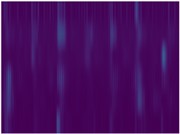
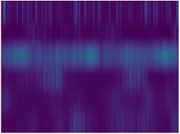
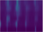
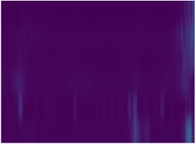
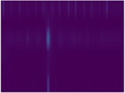
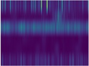
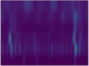
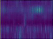
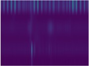
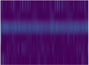
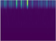
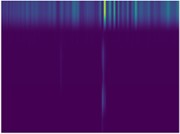
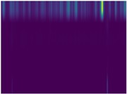
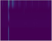
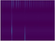
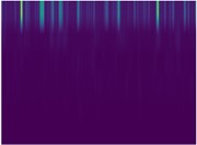
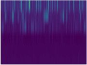
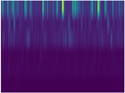
The feature images generated from two different fault datasets are presented in Figs. 3-4, respectively. Among them, Fig. 3 shows the feature images corresponding to three different fault types (with varying damage diameters) under the bearing speed condition of 1750 r/min. Fig. 4 displays twelve categories of fault feature images under each speed condition, covering inner race faults, outer race faults, ball faults, and normal state data.

As analyzed from Figs. 3-4, the proposed PVIE image encoding method can not only clearly characterize the discriminative features in fault data but also effectively suppress redundant feature interference. This redundancy suppression effect helps avoid the performance degradation of the diagnostic model caused by feature redundancy, providing support for the accuracy of fault diagnosis.

Fig. 2Schematic diagram of feature image generation

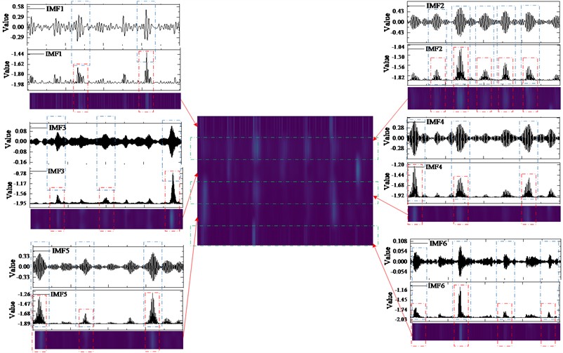
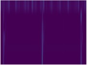
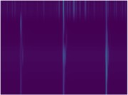
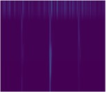
Fig. 3Schematic diagram of CWRU fault data feature images encoded by PVIE under 1750 r/min: a) Normal; b)-d) Inner race faults with increasing diameters; e)-g) Outer race faults with increasing diameters; h)-j) Rolling element faults with increasing diameters. It can be observed that as the fault diameter increases, the texture in the images becomes coarser and the color contrast intensifies, particularly evident in the diagonal patterns

Schematic diagram of CWRU fault data feature images encoded by PVIE under 1750 r/min: a) Normal; b)-d) Inner race faults with increasing diameters; e)-g) Outer race faults with increasing diameters; h)-j) Rolling element faults with increasing diameters. It can be observed that as the fault diameter increases, the texture in the images becomes coarser and the color contrast intensifies, particularly evident in the diagonal patterns

a)

b)

c)

d)

e)

f)

g)

h)

i)

j)

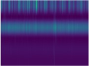
Fig. 4Schematic diagram of JN fault data feature images encoded by PVIE: a)-c) 600, 800, 1000 rpm under normal state; d)-f) 600, 800, 1000 rpm under inner race fault state; g)-i) 600, 800, 1000 rpm under outer race fault state; j)-l) 600, 800, 1000 rpm under roller fault state. Distinct differences in image structure and color distribution can be seen across different fault types, demonstrating the discriminative capability of PVIE

Schematic diagram of JN fault data feature images encoded by PVIE: a)-c) 600, 800, 1000 rpm under normal state; d)-f) 600, 800, 1000 rpm under inner race fault state; g)-i) 600, 800, 1000 rpm under outer race fault state; j)-l) 600, 800, 1000 rpm under roller fault state. Distinct differences in image structure and color distribution can be seen across different fault types, demonstrating the discriminative capability of PVIE

a)

b)

c)

d)

e)

f)

g)

h)

i)

j)

k)

l)

4. Model performance verification experiment

Multi-condition bearing fault data was segmented using a non-overlapping data window of specified size. The segmented sub-data was converted into fault feature images via PVIE, which were ultimately used to construct the fault dataset. The data window size set in this study was 2048, and the results of feature image generation for different datasets are as follows: the CWRU fault dataset contains 30 fault types, with each fault type corresponding to 238 feature images, resulting in a total dataset size of 7140 images. The JN fault dataset covers 12 fault types, with each fault type generating 244 feature images, and the total scale of the dataset is 2928 images. To ensure the fairness of the comparative experiment, all the image encoding methods involved in the comparison (including GADF, GASF, MTF, RP and the PVIE method proposed in this paper) follow exactly the same signal preprocessing procedure: the original vibration signal is first decomposed by VMD to obtain a set of IMF components. Then, each method encodes the image based on the same set of IMF components to generate fault feature maps. This approach aims to strictly control the variables, so that the performance differences are entirely attributed to the representation capabilities of the different encoding methods for the features, rather than the differences in the preprocessing steps.

The constructed multi-condition bearing fault dataset was divided into Subset A and Subset B at an 8:2 ratio, where Subset B was fixed as the model validation set. During the model training phase, Subset A was further split into training and testing sets to explore the influence of reduced training set size on the diagnostic performance of the model. It should be specifically noted that when adjusting the division ratio of the training set and testing set in subsequent experiments, the number of samples in the validation set (Subset B) remained unchanged.

The diagnostic results of the model on the two multi-condition bearing fault datasets are shown in Figs. 5-6, respectively. To verify the superiority of the diagnostic performance of the proposed PVIE method, a variety of commonly used feature image conversion methods were introduced for comparative experiments, and the input data of all comparative experiments were preprocessed by VMD. Meanwhile, small-scale data diagnostic experiments were designed to analyze the impact of data volume on model performance: for the CWRU dataset, after dividing the samples of each fault type into Subsets A and B at an 8:2 ratio, Subset B (validation set) contained 48 feature images for each fault type; the 190 feature images in Subset A were divided into training and testing sets according to different ratios, where the number of training set samples was 133 (70 %), 57 (30 %), and 19 (10 %) respectively. For the JN dataset, under the same ratio settings, the number of feature images corresponding to the training set was 136 (70 %), 59 (30 %), and 20 (10 %), respectively.

Firstly, the influence of VMD decomposition layers on diagnostic performance was analyzed, and the effectiveness of the PVIE method was verified. Two comparative scenarios were set up in the experiment: (1) directly converting the features of the CWRU dataset decomposed by VMD with different layers into heatmaps; (2) under the same VMD decomposition layers, using the PVIE method to convert the decomposed features into images.

The diagnostic results of the two scenarios are shown in Table 3, where VMD3W represents that the number of VMD decomposition layers is set to 3.

Table 3The number of different decomposition layers and the experimental results of PVIE validity verification

Method	Accuracy	Method	Accuracy
VMD3W	80.29 %	VMD5W	89.22 %
VMD3W-PVIE	98.64 %	VMD5W-PVIE	99.71 %
VMD4W	79.08 %	VMD6W	87.65 %
VMD4W-PVIE	99.00 %	VMD6W-PVIE	99.92 %

As presented in Table 3, it can be observed that the model’s fault diagnostic accuracy improves with an increase in the number of VMD decomposition layers. However, when the number of decomposition layers reaches 6, a decline in diagnostic accuracy is observed. It is worth noting that when the decomposition layer $K$ of VMD exceeds 6, the diagnostic accuracy of directly converting the VMD decomposition results into a heat map decreases. The physical mechanism behind this is that an excessively high decomposition layer ( $K >$ 6) disrupts the intrinsic modal structure of the signal and introduces over-decomposition and modal aliasing phenomena. Modal aliasing causes the fault features to be dispersed into multiple adjacent IMF components, which disrupts the integrity and clarity of the features in a single mode, resulting in the image obtained through direct encoding containing blurry and redundant information, thereby reducing the diagnostic accuracy. In contrast, the proposed PVIE method (VMD6W-PVIE) can still achieve an extremely high accuracy of 99.92 % in this situation. This is because the PWEDFE module in PVIE plays a crucial role. It can re-integrate and enhance the periodic impact features related to the fault through its weighted Euler difference operation from multiple aliased IMF components, while suppressing the non-correlated modal components generated by over-decomposition. Therefore, even when VMD decomposition is not optimal, PVIE can effectively “filter” and "extract" the most essential discriminative features, ensuring the quality of image encoding and the robustness of subsequent diagnosis. Consequently, 6 layers were selected as the optimal parameter for VMD decomposition in this study. Furthermore, the aforementioned experiments further validate the effectiveness of PVIE in the field of bearing fault diagnosis.

4.1. Multi-condition bearing fault diagnosis experiment

When conducting fault diagnosis using the CWRU fault dataset, the proposed PVIE method achieved an average diagnostic accuracy of 99.67 % across three different scales. This accuracy represents improvements of 36.96 %, 33.18 %, 51.29 %, and 50.13 % compared with those of the comparison methods. When the JNU dataset was used for diagnosis, the proposed method attained an average diagnostic accuracy of 99.00 % across the same three scales, demonstrating improvements of 31.11 %, 38.00 %, 42.02 %, and 37.82 % relative to the compared image encoding methods.

More notably, the proposed method also achieves significant advancements in image lightweighting. For example, during the diagnostic process – when the model was validated on the validation set – the diagnostic time corresponding to validation sets constructed by different image encoding methods is presented in Table 4. In this experiment, the division ratio of the training set to the test set was set to 8:2, with the test set accounting for 20 % of all generated fault images. Specifically, the multi-condition fault diagnosis time of the proposed method on the CWRU dataset is only 21 seconds, which is a substantial reduction compared with that of the comparison methods. This result further confirms the lightweight characteristic of PVIE.

Fig. 5Experimental results of CWRU data set under different image conversion methods

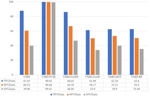
Fig. 6Experimental results of JN data set under different image conversion methods

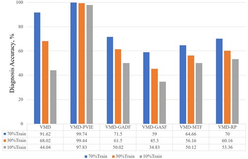
Table 4Comparison of time required for model diagnosis

Method	PVIE	GADF	GASF	MTF	RP
Time / s	21	262	73	79	45

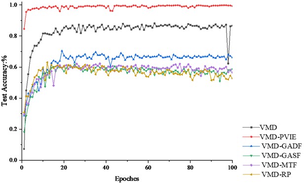
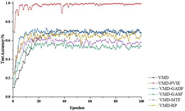
Additionally, the training process of the diagnostic model was visualized under the scenario where the training set accounts for 70 % of the total data. Figs. 7-10 illustrate the training and testing processes of the model for fault diagnosis using the CWRU bearing fault dataset. It can be observed that the AlexNet model achieves convergence irrespective of the image encoding method employed to transform the bearing fault data. Nevertheless, the models exhibit low accuracy in the testing phase, and only the diagnostic model trained on images converted via PVIE maintains stable convergence while ensuring reliable diagnostic performance.

Fig. 7Training accuracy of CWRU dataset diagnostic

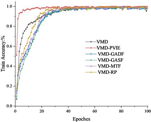
Fig. 8Testing accuracy of CWRU dataset diagnostic

4.2. Diagnostic experiment under noise condition

When bearings are in actual operation, the bearing data are inevitably disturbed by noise during acquisition, which impacts the fault diagnosis performance of the model. In this paper, Gaussian white noise with different signal-to-noise (SNR) ratios was added to the original vibration signal to simulate the noise environment in actual operating conditions, and fault diagnosis experiments were conducted using the added noise data to verify the noise immunity of the model. In this paper, the SNR was used as a measure of the noise level, which is defined in Eq. (14):

14

S N R = 10 \lg (\frac{P_{s}}{P_{n}}),

where $P_{s}$ is the signal power and $P_{n}$ is the noise power. When the diagnostic object is the CWRU fault data, using PVIE to convert fault data with added noise levels of –6 db, –12 db, and –18 db, the results was shown in Tables 5-7, the model achieved diagnostic accuracies of 99.85 %, 99.17 %, and 99.73 %, respectively. These results represent improvements of 13.82 %, 73.94 %, and 77.38 %, respectively, over the GADF method. Even when the training data size is reduced, the proposed method maintains high diagnostic accuracy.

Fig. 9Training accuracy of JN dataset diagnostic

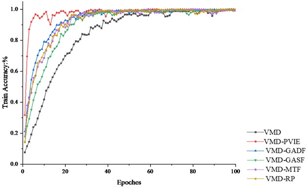
Fig. 10Testing accuracy of JN dataset diagnostic

When the diagnostic object is the JN fault data, the results were shown in Tables 8-10, the proposed method achieved 100 % diagnostic accuracy with added –6 db noise across three different data scales. When the noise level increased to -18db, the diagnostic model still achieved 98.83 % accuracy using PVIE as the image conversion method, while the results of the comparison methods did not exceed 25 %.

Table 5–6 db noise CWRU fault dataset diagnosis results

CWRU (–6 db)	VMD	VMD-PVIE	VMD-GADF	VMD-GASF	VMD-MTF	VMD-RP
70 % train	71.94 %	99.85 %	86.03 %	61.09 %	62.38 %	62.80 %
30 % train	32.09 %	98.34 %	66.58 %	50.17 %	53.31 %	50.40 %
10 % train	28.66 %	94.53 %	46.86 %	33.90 %	39.90 %	35.44 %
Average	44.23 %	97.57 %	66.49 %	48.38 %	51.86 %	49.54 %

Table 6–12 db noise CWRU fault dataset diagnosis results

CWRU (–12 db)	VMD	VMD-PVIE	VMD-GADF	VMD-GASF	VMD-MTF	VMD-RP
70 % train	61.12 %	99.17 %	25.23 %	17.67 %	19.51 %	21.08 %
30 % train	38.16 %	98.03 %	20.98 %	14.29 %	17.23 %	18.65 %
10 % train	26.62 %	92.51 %	17.47 %	10.58 %	13.16 %	14.17 %
Average	41.96 %	96.57 %	21.22 %	14.18 %	16.63 %	17.96 %

Table 7–18 db noise CWRU fault dataset diagnosis results

CWRU (–18 db)	VMD	VMD-PVIE	VMD-GADF	VMD-GASF	VMD-MTF	VMD-RP
70 % train	3.33 %	99.73 %	22.35 %	13.95 %	16.69 %	19.35 %
30 % train	3.42 %	98.87 %	19.37 %	10.63 %	14.29 %	17.38 %
10 % train	3.19 %	90.98 %	12.25 %	8.34 %	11.87 %	14.43 %
Average	3.31 %	96.52 %	17.99 %	10.97 %	14.28 %	17.05 %

Table 8–6 db noise JN fault dataset diagnosis results

JN (–6 db)	VMD	VMD-PVIE	VMD-GADF	VMD-GASF	VMD-MTF	VMD-RP
70 % train	84.35 %	100 %	71.5 %	59 %	64.66 %	70 %
30 % train	49.19 %	100 %	61.5 %	45.3 %	56.16 %	60.16 %
10 % train	32.99 %	100 %	50.02 %	34.83 %	50.12 %	53.36 %
Average	55.51 %	100 %	61 %	46.37 %	56.98 %	61.17 %

Table 9–12 db noise JN fault dataset diagnosis results

JN (–12 db)	VMD	VMD-PVIE	VMD-GADF	VMD-GASF	VMD-MTF	VMD-RP
70 % train	31 %	100 %	43.66 %	28.33 %	31.33 %	33 %
30 % train	22.5 %	100 %	34 %	24 %	27.83 %	27.33 %
10 % train	19.66 %	99.83 %	27.65 %	21.09 %	24.19 %	21.95 %
Average	24.38	99.94 %	35.1 %	24.47 %	27.78 %	27.42 %

Table 10–18 db noise JN fault dataset diagnosis results

JN (–18 db)	VMD	VMD-PVIE	VMD-GADF	VMD-GASF	VMD-MTF	VMD-RP
70 % train	26.83 %	99.66 %	28 %	8.33 %	26 %	17.33 %
30 % train	23.44 %	98.33 %	22.16 %	8.33 %	23 %	14.16 %
10 % train	19.07 %	98.5 %	19.66 %	8.33 %	19.33 %	8.33 %
Average	23.11 %	98.83 %	23.27 %	8.33 %	22.77 %	13.27 %

To further verify the superiority of the method proposed in this paper, we compared it with some other literature that uses feature image coding methods. The fault dataset used is CWRU. The dataset division is maintained at 20 % of the total data as the validation set, and the remaining data is divided into the training set and the test set in a 7:3 ratio. The final diagnosis results are shown in Table 11.

As can be seen from Table 11, compared with other diagnostic methods, the method proposed in this paper still maintains relatively stable diagnostic performance under strong noise interference.

Table 11The result of comparison with other methods

	–6 db data	–12 db data	–18 db data
REF [21]	97.81 %	93.37 %	80.29 %
REF [23]	99.21 %	97.53 %	90.08 %
REF [25]	98.72 %	94.16 %	88.40 %
Ours	99.85 %	99.17 %	99.73 %

5. Discussion

The PVIE method proposed in this study, compared with the existing image encoding-based fault diagnosis methods, has a core breakthrough in that it actively enhances the fault discrimination features under multiple operating conditions through PWEDFE, and achieves lightweight feature maps by relying on the Viridis mapping. This solves the problems of poor feature separability and low diagnostic efficiency of traditional methods. Moreover, through the synergy of VMD noise reduction and feature enhancement, the diagnostic robustness in strong noise and small sample scenarios has been significantly improved. This is also the key reason why its diagnostic accuracy and efficiency are significantly superior to methods such as GADF, GASF, MTF, and RP. Experimental results show that the matching degree between the number of VMD decomposition layers and the complexity of fault signal features directly affects the diagnostic effect. The 6-layer configuration is the optimal parameter for this experiment. This rule can provide a reference for similar bearing signal processing. However, this method still has limitations such as the need for manual experimentation to determine VMD parameters and the absence of multi-sensor data fusion. In the future, it can be combined with intelligent optimization algorithms to achieve adaptive selection of VMD parameters and further enhance the universality and engineering adaptability of the method by integrating multi-sensor signals.

6. Conclusions

To address the core challenges in multi-condition bearing fault diagnosis – specifically, the inability of existing image encoding methods to effectively distinguish fault features across varying operating conditions, and the high complexity and redundancy of current feature images that hinder diagnostic efficiency – this paper proposed a novel feature image encoding method based on PVIE. The implementation framework proceeded as follows: first, VMD was employed to decompose the raw bearing fault data; second, the decomposed components were transformed into feature images using the proposed PVIE method; finally, these images were fed into an AlexNet network model to achieve accurate fault diagnosis under multi-condition scenarios. The main contributions of this study are summarized as follows:

1) A lightweight fault feature encoding method, termed PVIE, was proposed. This method realizes effective extraction of discriminative fault features through the PWEDFE module, thereby ensuring the representational validity of the image encoding. Simultaneously, it achieves lightweight compression of feature images via the VFVM mechanism, significantly reducing the computational load for subsequent models.

2) Experimental results demonstrated that the multi-condition bearing fault encoding scheme integrating VMD and PVIE exhibits superior encoding performance. Further verification confirmed that the proposed method maintains robust diagnostic accuracy even under strong noise interference and small-sample scenarios, highlighting its significant potential for engineering applications.

3) The intrinsic relationship between the feature extraction performance of the diagnostic model and the dominance of fault representation within the feature images was revealed. The study found that the VMD-based feature extraction process is highly sensitive to the settings of penalty and modal parameters; improper parameter selection prone to inducing modal aliasing. Such aliasing effects lead to deviations in feature extraction, resulting in incomplete and ambiguous fault information expression in the generated images, which ultimately causes diagnostic errors.

References

Z. Ma, S. Wang, J. Shi, T. Li, and X. Wang, “Fault diagnosis of an intelligent hydraulic pump based on a nonlinear unknown input observer,” Chinese Journal of Aeronautics, Vol. 31, No. 2, pp. 385–394, Feb. 2018, https://doi.org/10.1016/j.cja.2017.05.004

Publisher
D.-T. Hoang and H.-J. Kang, “A survey on deep learning based bearing fault diagnosis,” Neurocomputing, Vol. 335, pp. 327–335, Mar. 2019, https://doi.org/10.1016/j.neucom.2018.06.078

Publisher
Y. Q. Lu, “Research on compound fault diagnosis method of planetary gearbox based on convolutional neural network,” University of Electronics Science and Technology of China, 2020.

Search CrossRef
J. Zheng, H. Pan, Q. Liu, and K. Ding, “Refined time-shift multiscale normalised dispersion entropy and its application to fault diagnosis of rolling bearing,” Physica A: Statistical Mechanics and its Applications, Vol. 545, p. 123641, May 2020, https://doi.org/10.1016/j.physa.2019.123641

Publisher
J. Wang, Q. B. He, and K. R. Kong, “Adaptive multiscale noise tuning stochastic resonance for health diagnosis of rolling element bearings,” IEEE Transactions on Instrumentation and Measurement, Vol. 64, No. 2, pp. 564–577, Feb. 2015, https://doi.org/10.1109/tim.2014.2347217

Publisher
Q. Xue et al., “Feature extraction using hierarchical dispersion entropy for rolling bearing fault diagnosis,” IEEE Transactions on Instrumentation and Measurement, Vol. 70, pp. 1–11, Jan. 2021, https://doi.org/10.1109/tim.2021.3092513

Publisher
L. Song, H. Wang, and P. Chen, “Vibration-based intelligent fault diagnosis for roller bearings in low-speed rotating machinery,” IEEE Transactions on Instrumentation and Measurement, Vol. 67, No. 8, pp. 1887–1899, Aug. 2018, https://doi.org/10.1109/tim.2018.2806984

Publisher
H. Li et al., “Composite fault diagnosis for rolling bearing based on parameter-optimized VMD,” Measurement, Vol. 201, p. 111637, Sep. 2022, https://doi.org/10.1016/j.measurement.2022.111637

Publisher
Z. Jin, D. He, and Z. Wei, “Intelligent fault diagnosis of train axle box bearing based on parameter optimization VMD and improved DBN,” Engineering Applications of Artificial Intelligence, Vol. 110, p. 104713, Apr. 2022, https://doi.org/10.1016/j.engappai.2022.104713

Publisher
C. B. He et al., “Signal denoising method based on parametric self-optimizing VMD,” (in Chinese), Journal of Vibration and Shock, Vol. 42, No. 19, pp. 283–293, 2022, https://doi.org/10.13465/j.cnki.jvs.2023.19.036

Publisher
C. L. Lei et al., “Rolling bearing fault diagnosis method based on SSA-IWT-EMD,” (in Chinese), Journal of Beijing University of Aeronautics and Astronautics, Vol. 51, No. 4, pp. 1–19, 2025, https://doi.org/10.13700/j.bh.1001-5965.2023.0174

Publisher
X. Y. Cong et al., “Identification of coal-rock interface based on EMD and kurtosis filter,” (in Chinese), Vibration Measurement and Diagnosis, Vol. 35, No. 5, pp. 950–954, 2015, https://doi.org/10.16450/j.cnki.issn.1004-6801.2015.05.024

Publisher
H. Zhao, H. Liu, J. Xu, C. Guo, and W. Deng, “Research on a fault diagnosis method of rolling bearings using variation mode decomposition and deep belief network,” Journal of Mechanical Science and Technology, Vol. 33, No. 9, pp. 4165–4172, Sep. 2019, https://doi.org/10.1007/s12206-019-0811-2

Publisher
H. Shao, M. Xia, J. Wan, and C. W. de Silva, “Modified stacked autoencoder using adaptive Morlet wavelet for intelligent fault diagnosis of rotating machinery,” IEEE/ASME Transactions on Mechatronics, Vol. 27, No. 1, pp. 24–33, Feb. 2022, https://doi.org/10.1109/tmech.2021.3058061

Publisher
C. L. Zhang et al., “Fault transients extraction of rolling bearings under varying speed via modified continuous wavelet transform enhanced nonconvex sparse representation,” Journal of Mechanical Engineering, Vol. 61, No. 1, p. 172, 2025, https://doi.org/10.3901/jme.2025.01.172

Publisher
W. Pan, H. Qu, Y. Sun, and M. Wang, “A deep convolutional neural network model with two-stream feature fusion and cross-load adaptive characteristics for fault diagnosis,” Measurement Science and Technology, Vol. 34, No. 9, p. 095102, Sep. 2023, https://doi.org/10.1088/1361-6501/acd01e

Publisher
Y. X. Wang et al., “Intelligent diagnosis for GIS with small samples using a novel adversarial transfer learning in convolutional neural network,” (in Chinese), Transactions of China Electrotechnical Society, Vol. 37, No. 9, pp. 2150–2160, 2022, https://doi.org/10.19595/j.cnki.1000-6753.tces.211512

Publisher
Z. Wang et al., “Two stage insulator fault detection method based on collaborative deep learning,” (in Chinese), Transactions of China Electrotechnical Society, Vol. 36, No. 17, pp. 3594–3604, 2021, https://doi.org/10.19595/j.cnki.1000-6753.tces.201320

Publisher
W. B. Bian et al., “Fault diagnosis method of wind turbine rolling bearing based on improved deep residual shrinkage network,” Journal of Mechanical Engineering, Vol. 59, No. 12, p. 202, Jan. 2023, https://doi.org/10.3901/jme.2023.12.202

Publisher
P. Wang, D. Q. Li, and H. Wang, “Rolling bearing fault diagnosis algorithm based on improved alternating transfer learning,” (in Chinese), Journal of Vibration and Shock, Vol. 43, No. 5, pp. 239–249, 2024, https://doi.org/10.13465/j.cnki.jvs.2024.05.026

Publisher
Y. Tong, X. Y. Pang, and Z. H. Wei, “Fault diagnosis method of rolling bearing based on GADF-CNN,” (in Chinese), Journal of Vibration and Shock, Vol. 40, No. 5, pp. 247–260, 2020, https://doi.org/10.13465/j.cnki.jvs.2021.05.032

Publisher
H. P. Liang, J. Cao, and X. Q. Zhao, “Small sample fault diagnosis method for rotating machinery based on GADF and PAM-Resnet,” (in Chinese), Control and Decision, Vol. 38, No. 12, pp. 3465–3472, 2023, https://doi.org/10.13195/j.kzyjc.2022.0378

Publisher
X. Y. Duan et al., “A rolling bearing fault diagnosis method based on MTF-MSMCNN with small sample,” (in Chinese), Journal of Aerospace Power, Vol. 39, No. 1, pp. 240–252, 2024, https://doi.org/10.13224/j.cnki.jasp.20230517

Publisher
M. X. Jiao et al., “Fault diagnosis method of small sample rolling bearing under variable working conditions based on MTF-SPCNN,” (in Chinese), Journal of Beijing University of Aeronautics and Astronautics, Vol. 50, No. 12, pp. 3696–3708, 2024, https://doi.org/10.13700/j.bh.1001-5965.2022.0927

Publisher
L. Zhang et al., “Fault diagnosis of rolling bearings using recurrence plot coding technique and residual network,” Journal of Xian Jiaotong University, Vol. 57, No. 2, pp. 110–120, 2023.

Search CrossRef
Y. Zhou, Z. Wang, X. Zuo, and H. Zhao, “Identification of wear mechanisms of main bearings of marine diesel engine using recurrence plot based on CNN model,” Wear, Vol. 520-521, p. 204656, May 2023, https://doi.org/10.1016/j.wear.2023.204656

Publisher

About this article

Received

January 6, 2026

Accepted

April 14, 2026

Published

June 4, 2026

SUBJECTS

Fault diagnosis based on vibration signal analysis

DOI

https://doi.org/10.21595/jve.2026.25992

Keywords

multistate

bearing

fault diagnosis

image encoding

lightweight

Acknowledgements

This study was funded by the Youth Innovation Team Development Plan of Higher Education Institutions in Shandong Province, CHINA, grant number 2025KJH100.

Data Availability

The datasets generated during and/or analyzed during the current study are available from the corresponding author on reasonable request.

Author Contributions

Xiaomin Teng: conceptualization, methodology, writing-original draft, funding acquisition. Huiying Xing: investigation, data curation, formal analysis. Wansheng Wang: supervision, project administration, writing-review and editing. Jing Li: software, validation, visualization. Yunlin Ma: resources, investigation, writing-review and editing.

Conflict of interest

The authors declare that they have no conflict of interest.

This is an open access article distributed under the Creative Commons Attribution License, which permits unrestricted use, distribution, and reproduction in any medium, provided the original work is properly cited.

X. Teng, H. Xing, W. Wang, J. Li, and Y. Ma, “A feature lightweight image coding method for fault diagnosis of hydraulic motor bearings: PVIE,” Journal of Vibroengineering, Vol. 28, No. 2, –17, Jun. 2026, https://doi.org/10.21595/jve.2026.25992

Copy Extrica

Copied to clipboard!

TY  - JOUR
DO  - 10.21595/jve.2026.25992
UR  - https://doi.org/10.21595/jve.2026.25992
TI  - A feature lightweight image coding method for fault diagnosis of hydraulic motor bearings: PVIE
T2  - Journal of Vibroengineering
AU  - Teng, Xiaomin
AU  - Xing, Huiying
AU  - Wang, Wansheng
AU  - Li, Jing
AU  - Ma, Yunlin
PY  - 2026
DA  - 2026/06/04
PB  - Extrica
VL  - 28
IS  - 2
SN  - 1392-8716
SN  - 2538-8460
ER  - 

Copy Ris

Copied to clipboard!

@article{doi_10.21595/jve.2026.25992,
  title = {A feature lightweight image coding method for fault diagnosis of hydraulic motor bearings: PVIE},
  author = {Teng, Xiaomin and Xing, Huiying and Wang, Wansheng and Li, Jing and Ma, Yunlin},
  journal = {Journal of Vibroengineering},
  year = {2026},
  month = {6},
  volume = {28},
  number = {2},
  doi = {10.21595/jve.2026.25992},
  url = {https://doi.org/10.21595/jve.2026.25992},
  publisher = {Extrica},
  issn = {1392-8716},
  eissn = {2538-8460},
}

Copy Bibtex

Copied to clipboard!

[1]X. Teng, H. Xing, W. Wang, J. Li, and Y. Ma, “A feature lightweight image coding method for fault diagnosis of hydraulic motor bearings: PVIE,” Journal of Vibroengineering, Jun. 2026, doi: 10.21595/jve.2026.25992.

Copy IEEE

Copied to clipboard!

Teng, Xiaomin, Huiying Xing, Wansheng Wang, Jing Li, and Yunlin Ma. “A feature lightweight image coding method for fault diagnosis of hydraulic motor bearings: PVIE.” Journal of Vibroengineering 28, no. 2 (2026). https://doi.org/10.21595/jve.2026.25992.

Copy Chicago

Copied to clipboard!