Abstract
A stranded wire helical spring is a cylindrical helical spring wound by a wire strand. Owing to its unique structure, the spring features special dynamic behavior such as nonlinear stiffness, hysteresis and hardening overlap. The dynamic response model, which gives an accurate description of the dynamic behavior, of the spring is a very important tool for designing systems using the spring as well as evaluating the responses of such systems. However, no accurate model has been reported. In the present study, a modified normalized Bouc-Wen model is proposed to model the dynamic behavior of the spring. A simple yet effective identification method is developed for identifying the model parameters using experimental data. Numerical simulations and periodic loading experiments were carried out to validate the proposed model and identification method. The results verify that the proposed model and method are effective for modeling and identifying the dynamic behavior of stranded wire helical springs.
1. Introduction
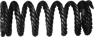
A stranded wire helical spring (see Fig. 1) is a cylindrical helical spring wound by a wire strand. The strand is usually composed of several layers of steel wires which are wrapped around an optional core wire or the axis of the strand. The core wire may be metallic materials, synthetic materials or natural fibers. The spring was first observed in machine guns [1]. Compared to conventional single wire springs, the stranded wire helical spring demonstrates longer fatigue life and better vibration absorption ability [2, 3]. Owing to its many advantages, the spring is widely used in automatic weapons, aircraft engines, metallurgical equipment, etc. as key vibration absorption components.
Fig. 1A stranded wire helical spring
Most studies regarding the spring have been focused on its manufacturing and geometric modeling. Wang et al [4] studied the dynamic tension on the wires during the manufacturing process. Peng et al [5] proposed a framework for designing the machine tool for the spring. Zhou et al [6] modeled the geometry of the spring using the double helix model.
The mechanical model of the spring is a very important tool for designing systems using the spring as well as evaluating the responses of such systems. However, due to the complexity of the structure of the spring, the mechanical modeling is rather difficult. Costello et al [1] proposed a theoretical model for determining the static response of the spring and the model was later generalized by Philips et al [7]. Costello and Phillips’ models were deduced from Love’s thin rod theory [8]. In their models, the unevenly distributed gaps between adjacent wires and the contact deformations of individual wires were ignored. As a result, these theoretical models can only give acceptable results for stranded wire helical springs under small axial deformations. Moreover, the friction between adjacent wires was also neglected in their analyses; hence, these models are not capable of modeling the damping behavior of the spring. On the other hand, the dynamic response of the spring is also seldom studied. To our knowledge, no accurate model has been reported.
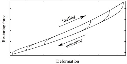
Owing to the friction between adjacent wires and the inter-wire contact deformation, hysteresis loops can be observed when the spring is under dynamic loads and the stiffness of the spring exhibits evident nonlinearity (see Fig. 2). For a stranded wire helical spring under axial compression or tension loads, the stiffness of the spring tends to increase with the deformation. Moreover, the loading paths of hysteresis loops with different amplitudes are almost overlapped. Such phenomenon is defined as the hardening overlap behavior [9]. To model hysteretic systems, a combined nth-power velocity and Coulomb friction damping model was proposed by Tinker et al [10]. With this model, the response of a hysteretic system is related to the velocity under which the component is excited. However, many studies have shown that the response of wire products are rate independent [11-13] and therefore this model suffers from several defects [9]. Hu et al [14] proposed a bilinear model for hysteresis. This model is suitable for modeling some systems with dry friction damping; however, it cannot describe the response of a stranded wire helical spring with high accuracy. A differential model was proposed by Bouc [15] and later generalized by Wen [16]. By setting different model parameters, the Bouc-Wen model is able to describe various kinds of hysteric systems with relative high accuracy. Nevertheless, the Bouc-Wen model is still unable to model the dynamic behavior of the spring properly for it cannot give a reasonable description of hysteretic systems with hardening overlap behavior. However, this problem could be coped with by introducing several modifications [9]. In practice, the parameters of the Bouc-Wen model and its modified versions are usually identified using experimental data. To this end, many identification methods were developed. These methods include time domain least square method [17-19], frequency domain least square method [20, 21], extended Kalman filtering technique [22, 23] and adaptive algorithm [24]. Iteration algorithms are adopted in most existing identification methods to search for the optimal parameters; hence, in order to use these methods, a set of initial values has to be manually chosen. However, the reasonable initial values may not be easy to find in practice and convergence problems are liable to occur. Ikhouane et al proposed a normalized Bouc-Wen model [25] along with a limit cycle identification method [26]. This method does not rely on iteration algorithms and therefore is free of convergence problems.
Fig. 2The typical dynamic response of a stranded wire helical spring
In the present work, a modified normalized Bouc-Wen model is proposed to describe the dynamic behavior of the stranded wire helical spring. A two-stage identification method, which involves no iteration procedures, is developed to identify the model parameters using experimental data. The model and the identification method are compared with another model and method [9, 21] in numerical simulations. Periodic loading experiments are conducted on a stranded wire helical spring. The results verify that the proposed model and identification method is effective for describing the dynamic behavior of the spring.
2. Modeling
2.1. Illustration and analysis of the Bouc-Wen model
The classic Bouc-Wen model is given by [16]:
where , and are the deformation, pure hysteretic restoring force and overall restoring force respectively. The term is an elastic component. The dot over , and denotes the derivation with respect to the time . , , , , , and are the model parameters to be identified and , , , are positive numbers.
A certain response of the Bouc-Wen model can be described by multiple sets of model parameters [25]. This is a problem for parameter identification. A normalized Bouc-Wen model was proposed by Ikhouane et.al [25] to cope with this problem. The normalized Bouc-Wen model is given in the form:
where , , , . is the pure hysteretic component of the normalized Bouc-Wen model while is the linear elastic component. The constant is given as:
The normalized Bouc-Wen model defines a bijection between the model parameters and the model response.
Although the Bouc-Wen model has been widely used to describe many hysteretic systems, it fails to describe the dynamic behavior of the stranded wire helical spring for it is incapable of describing hysteresis loops with hardening overlap behavior. The reasons are as follows. Firstly, the Bouc-Wen model is symmetric in nature while a hysteresis loop with hardening behavior is asymmetric. However, this may not be a critical problem for one can use two sets of parameters to describe the loading and unloading curves respectively (see Fig. 3). Secondly, the quantity of is unbounded when the Bouc-Wen model is used to describe systems with hardening hysteresis loops [9] and therefore no overlap loading path can be observed (see Fig. 3).
Fig. 3Hysteresis loops with hardening behavior generated by using two sets of parameters: (a) the overall response, (b) the pure hysteretic component of the overall response
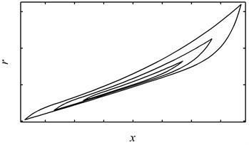
(a)
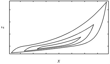
(b)
2.2. A modified Bouc-Wen model for stranded wire helical springs
The Bouc-Wen model can describe hysteresis loops with various shapes by using various combinations of parameters. However, only one class of combinations is physically possible, namely, the model is stable in the bounded input-bounded output (BIBO) sense and compatible with the laws of Thermodynamics. This combination requires [27]:
For the normalized Bouc-Wen model, Eq. (6) can be rewritten as:
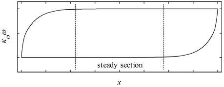
Under such a combination of parameters, the pure hysteretic component of the response will be bounded as depicted in Fig. 4. Moreover, the upper bound of the term is bounded to 1 and this suggests that the upper bound of the pure hysteretic component will be .
Fig. 4The pure hysteretic component generated by a set of physically possible parameters
To attain an asymmetric hysteresis loop, the pure hysteretic component of the normalized Bouc-Wen model is multiplied by a nonlinear amplifier. In this way, the overlap behavior can be guaranteed to be observed in the hysteresis loop for the amplitude of the pure hysteretic component is bounded. The nonlinear amplifier can be given by a polynomial:
where is the nonlinear amplifier, is the amplification coefficient and is the degree of the polynomial.
In order to give an accurate description of the nonlinear stiffness of the stranded wire helical spring, namely the hardening behavior, the linear elastic component of the Bouc-Wen model is replaced by a nonlinear elastic component:
where is the nonlinear elastic component, is the elastic coefficient and is the degree of the nonlinear component.
Combining the nonlinear elastic component, the nonlinear amplifier and the pure hysteretic component of the normalized Bouc-Wen model, the modified Bouc-Wen model for stranded wire helical springs is given as:
The values of and should be chosen according to the experimental data when identifying the parameters. For typical stranded wire helical springs, they are usually less than 4.
For the case , the term tends to infinity when approaches 0. This will lead to numerical problems when identifying the model parameters. Therefore, Eq. (4) is rewritten in the following form:
3. Identification of the model parameters
The identification procedure is divided into two stages in the present study. The parameters of the nonlinear elastic component and the nonlinear amplifier are identified in the first stage. Using the identification results, the pure hysteretic response is extracted from the overall response and then employed in the second stage to identify the parameters of the pure hysteretic component.
3.1. Stage 1: Identification of non-hysteretic parameters
Since the response of a physically possible pure hysteretic component, namely, the term , is bounded and symmetric with respect to the -axis when is in the "steady section" (see Fig. 4), the response in this section can be given as:
where is the upper or loading branch and is the lower or unloading branch of the hysteresis loop.
Owing to the fact that the experimental data is discontinuous, Eq. (12) should be recast as the discrete form:
where the subscript 1, 2, …, , denotes the th point of the discrete data and is the length of the discrete data.
To identify the parameters of , the response of the nonlinear elastic component must be extracted from the overall response first. By using Eq. (13), can be discretely derived as:
Eq. (9) can be rewritten as a discrete linear form:
where , is the nonlinear stiffness coefficients vector and is the linearized deformation vector.
An error function and an objective function can be given by Eqs. (16) and (17) respectively:
Eqs. (15)-(17) define a linear optimization problem. The solution to the problem, i.e. an optimal , can be derived using linear least square method [28] without any iteration procedures.
The parameters of the nonlinear amplifier can be derived through a similar process. The response of the nonlinear amplifier can be obtained discretely through Eq. (13) as:
The upper bound of the pure hysteretic component is actually a redundant variable which can be combined with the coefficients of . Assuming , then under such circumstances can be derived as:
where is an arbitrary point in the steady section and it can be chosen to be the average value of in a period for convenience.
Substituting Eq. (19) into Eq. (18), one has:
Define the nonlinear amplification coefficients vector as and the linearized deformation vector . An optimization problem similar to Eq. (17) can be derived and solved following the identification process of .
3.2. Stage 2: Identification of hysteretic parameters
The pure hysteretic response, i.e. the limit cycle of the pure hysteretic component can be extracted from the overall response through Eq. (10) and written in the discrete form as:
where is the extracted pure hysteretic restoring force.
The hysteretic parameters are identified using the extracted response following a limit cycle approach [26], which uses the implicit information within the experimental data.
Eq. (11) can be rewrite in a piecewise form:
The hysteretic parameter can be readily derived from Eqs. (21) and (22) as follows:
where is the point where 0.
The identification of the rest of the parameters can be performed on either branch of the extracted hysteresis loop. Let the symbol denote the minimal for the loading branch or the maxim for the unloading branch. Choose a point which meets the condition for the loading branch or for the unloading branch. Take another two points , which meet the condition for the loading branch or for the unloading branch. Substituting , into Eq. (22) and the parameter n can be solved for as:
The parameter can be identified by substituting along with the identified , and into Eq. (22) as:
Similar to the identification process of stage 1, no iterations are involved in this stage.
3.3. Processing of experimental data
The second stage of the identification process requires the calculation of the derivative of Ω with respect to x. Since the experimental data are discrete, the derivative is calculated using difference quotient. In practice, the measured data will inevitably be contaminated by noises, which will introduce significant error to the calculated derivative. Therefore, the measured data has to be processed before the identification process.
A simple yet effective way of denoising is the moving average method [29]. This method would be sufficient if the experimental data is not severely contaminated. For the case where the experimental data is severely contaminated, the data should be filtered using digital low pass filters first. For the data measured in a periodic loading experiment, an effective frequency domain non-causal filtering method proposed by Ni et al [20] could be adopted. The discrete Fourier series (DFS) is employed in this method to eliminate the high frequency noises and reconstruct the measured periodic signals.
4. Numerical simulation
Deformation controlled loading simulations are performed to verify the effectiveness of the present model and identification method. Ni et al [9] proposed another modified Bouc-Wen model (Ni's model for short) which is capable of modeling hysteretic system with nonlinear stiffness and hardening overlap behavior. The model is identified using a frequency domain identification method [21] (Ni's method for short). The simulated experimental data in the present simulations is produced by Ni's model. The present model and identification method and that of Ni's are adopted to model the simulated response respectively.
Ni’s model is given by [9]:
where , , , , , , and are model parameters. A set of parameters was presented by Ni et al [21] as: 39.145, 1.360, 0.156, 1.799, 0.202, 147.761, 15.512, 44.726.
Since the simulations are deformation controlled, i.e. the deformation x is given explicitly, is then given by simple sinusoidal signals:
where is the amplitude of the deformation.
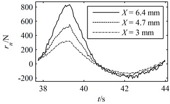
The term and are obtained by substituting the generated into Eqs. (27) and (28). Meanwhile, is also substituted into Eq. (29) and the term is readily calculated through solving the differential equation numerically. The "true" response is then given by Eq. (26). However, it should be noted that the actual experimental data would inevitably be contaminated by noises which will significantly affect the accuracy of the identification result. Hence, in order to simulate the actual experimental data, noises are introduced into the true response and the simulated experimental data is given in the following form [20] and presented in Fig. 5:
where is the ratio of noise to signal or the "noise level" and is a white noise signal. The noise level is set to 0.03 in the simulations.
The parameters of the present model and Ni's model are identified using the present identification method and Ni's method respectively. Since the Levenberg-Marquardt method, which is an iteration method, is employed in Ni's method to search for the optimal parameters, a set of initial values must be manually chosen. In the present simulation, two sets of initial trials are used. One of them is a sequence of randomly generated numbers and the other one is the exact values of the parameters. The predicted responses produced using the identified parameters and the true responses are presented in Figs. 6-8.
Fig. 5A period of the simulated experimental data: (a) the deformation and response in the time domain, (b) the hysteresis loop
(a)
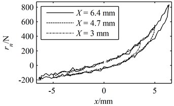
(b)
To quantify the goodness of the predicted responses, two statistics are calculated and presented in Table 1 for each prediction. One of them is the root mean square error () which is given by:
where is the discrete predicted response. The other one is a coefficient of determination for nonlinear models given by Zhang [30]:
Table 1The RMSE and RNL of the predicted hysteresis loops
Model | ||
The present model | 2.5337 | 0.98979 |
Ni's model (identified using random initial values) | 6.0202 | 0.97575 |
Ni's model (identified using exact initial values) | 2.0494 | 0.99174 |
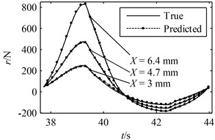
Fig. 6A period of the true responses and the predicted responses using parameters identified through the present method: (a) the responses in the time domain, (b) the hysteresis loops
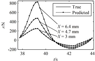
(a)
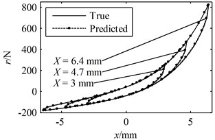
(b)
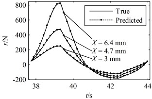
Fig. 7A period of the true responses and the predicted responses using parameters identified through Ni's method with random initial values: (a) the responses in the time domain, (b) the hysteresis loops
(a)

(b)
Fig. 8A period of the true responses and the predicted responses using parameters identified through Ni's method with exact initial values: (a) the responses in the time domain, (b) the hysteresis loops
(a)
(b)
A greater value indicates a better prediction while the closer the is to 1 the more accurate the predicted response is to the true response. According to Figs. 6-8 and Table 1, it can be concluded that all of the predicted responses are rather close to the true response. However, the values of and given in Table 1 clearly show that the present model and identification method is able to predict the responses with better accuracy compared with Ni's model with parameters identified using random initial values, even though the simulated experimental data was generated by Ni's model instead of the present model. On the other hand, in order for Ni's method to converge to a good solution, a set of suitable initial values must be given correctly. In fact, many sets of random initial values were tried in the simulations; however, most of them failed to converge to a reasonable solution. For the ones that did lead to convergence, it usually takes more than 100 iterations in the present simulation. Moreover, a FFT and an iFFT procedure are required by Ni's method in each iteration and therefore the method is rather time consuming. On the other hand, the most significant advantage of the present identification method is that no initial values are required and no iteration is involved. There are also no time consuming procedures in the identification process. Therefore, the computational efficiency of the present method is much higher than that of Ni's method. However, it should also be noted that the prediction made by the present model and method is not optimal compared with that of Ni's model and method provided that the exact parameter values are given as initial values. This is because of that no optimization problem is constructed in the second stage and therefore there is no guarantee that the identified parameters are optimum.
5. Experiment
Deformation controlled periodic loading experiments were carried out on a stranded wire helical spring and the present model and identification method are employed to model the dynamic response of the spring.
5.1. Setup of the experiment
The experiments are carried out on an electro-hydraulic servo vibration test rig (see Fig. 9). The spring is hold between two holding plates. A holding mandrel is inserted through the spring to keep it from being severely bent. The two holding plates are fixed by two clamps respectively. The upper clamp is fixed throughout the experiment while the lower one vibrates periodically in the axial direction to load the spring.
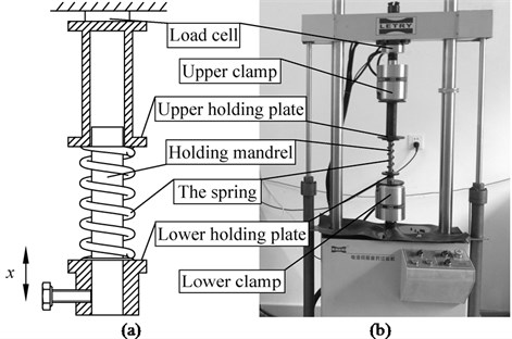
Fig. 9. Setup of the experiment: (a) schematic diagram, (b) the actual setup
In this way, the deformation of the spring is equivalent to the displacement of the lower clamp. The upper clamp is installed on top of a load cell. The displacement of the lower clamp is measured by a potentiometric linear displacement sensor. The restoring force and displacement signals are sampled synchronously. The periodic displacement of the lower clamp is set for the amplitude range 13-46 mm and for the frequency range 0.13-2.12 Hz.
The spring is composed of one core wire and two layers of outer wires. The external layer is composed of six wires and the middle layer is composed of three wires. The diameter of all the wires is 1.5 mm. The length of the spring is 176 mm. The spring under test is a compression spring, namely that the strand is wound in the opposite sense as that of the spring. It should be noted that, unlike single wire springs, a compression stranded wire helical spring is designed to resist compression loads only and should not be loaded with tension loads. Hence, a pre-deformation of 57 mm is applied to the spring and therefore the spring is under compression loads throughout the experiment process.
5.2. Results
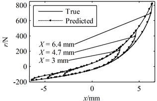
The experimentally measured hysteresis loops are illustrated in Fig. 10 along with the predicted hysteresis loops generated using the present model and the identified parameters. The and of the predicted hysteresis loops are presented in Table 2. It can be seen that the predicted and measured hysteresis loops coincide with each other well. In particular, the nonlinear stiffness and hardening overlapping behavior can be clearly observed.
Fig. 10The measured and predicted hysteresis loops
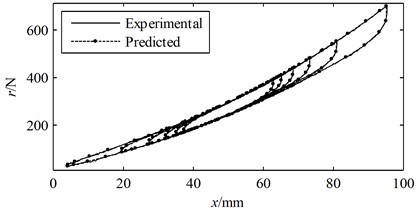
Table 2The RMSE and RNLof the predicted hysteresis loops
3.5523 | 0.98825 |
The experiments verify that the present model and identification method are effective for modeling the dynamic behavior of the stranded wire helical spring using dynamic loading experimental data.
6. Conclusions
A phenomenological model that is able to give an accurate description of the dynamic behavior of the stranded wire helical spring has been proposed in the present work. The model is a modified normalized Bouc-Wen model in essence. Making use of the knowledge of the shape of a hysteresis loop produced by the Bouc-Wen model using physically possible model parameters, the pure hysteretic component of the original Bouc-Wen model was introduced into the proposed model along with a nonlinear elastic component and a nonlinear amplifier. As a result, the model is capable of modeling hysteresis loops with nonlinear stiffness and hardening overlap behavior. A two-stage identification method was developed to identify the model parameters. The parameters regarding the nonlinear elastic component and the nonlinear amplifier were identified using linear least square method in the first stage of the identification process. The pure hysteretic response was extracted from the overall response and the hysteretic parameters were identified using a limit cycle approach in the second stage. The presented identification method does not involve any iteration procedure throughout the identification process; hence, no initial values are required and no convergence problems would occur. Moreover, the method is much more time saving compared with iteration methods. The effectiveness of the proposed model and identification method has been verified by numerical simulations and experiments. On the other hand, since no optimization problem was constructed in the identification process, the identification method does not guarantee an optimal estimation of the model parameters. Therefore, if optimal model parameters are required, the presented method can be employed first to find a set of model parameters and the identified parameters can be then used as initial values for conventional iteration methods. Such treatment would be helpful for the iteration methods to reach convergence.
References
-
Costello G. A., Phillips J. W. Static response of stranded wire helical springs. International Journal of Mechanical Sciences, Vol. 21, Issue 3, 1979, p. 171-178.
-
Wang S. L., Lei S., Zhou J., Xiao H. Mathematical model for determination of strand twist angle and diameter in stranded-wire helical springs. Journal of Mechanical Science and Technology, Vol. 24, Issue 6, 2010, p. 1203-1210.
-
Wang S. L., Li X. Y., Lei S., Zhou J., Yang Y. Research on torsional fretting wear behaviors and damage mechanisms of stranded-wire helical spring. Journal of Mechanical Science and Technology, Vol. 25, Issue 8, 2011, p. 2137-2147.
-
Wang S., Zhou J., Kang L. Dynamic tension of stranded wires helical spring during reeling. Chinese Journal of Mechanical Engineering, Vol. 44, Issue 6, 2008, p. 36-42.
-
Peng Y. X., Wang S. L., Zhou J., Lei S. Structural design, numerical simulation and control system of a machine tool for stranded wire helical springs. Journal of Manufacturing Systems, Vol. 31, Issue 1, 2012, p. 34-41.
-
Zhou J., Wang S. L., Kang L., Chen T. Y. Design and modeling on stranded wires helical springs. Chinese Journal of Mechanical Engineering, Vol. 24, Issue 4, 2011, p. 626-637.
-
Phillips J. W., Costello G. A. General axial response of stranded wire helical springs. International Journal of Non-Linear Mechanics, Vol. 14, Issue 4, 1979, p. 247-257.
-
Love A. E. H. A Treatise on the Mathematical Theory of Elasticity. New York: Courier Dover Publications, 1944.
-
Ni Y. Q., Ko J. M., Wong C. W., Zhan S. Modelling and identification of a wire-cable vibration isolator via a cyclic loading test, Part 1: Experiments and model development. Proceedings of the Institution of Mechanical Engineers, Part I – Journal of Systems and Control Engineering, Vol. 213, Issue 3, 1999, p. 163-171.
-
Tinker M. L., Cutchins M. A. Damping phenomena in a wire rope vibration isolation system. Journal of Sound and Vibration, Vol. 157, Issue 1, 1992, p. 7-18.
-
Demetriades G. F., Constantinou M. C., Reinhorn A. M. Study of wire rope systems for seismic protection of equipment in buildings. Engineering Structures, Vol. 15, Issue 5, 1993, p. 321-334.
-
Gerges R. R. Model for the force-displacement relationship of wire rope springs. Journal of Aerospace Engineering, Vol. 21, Issue 1, 2008, p. 1-9.
-
Ko J. M., Ni Y. Q., Tian Q. L. Hysteretic behavior and empirical modeling of a wire-cable vibration isolator. The International Journal of Analytical and Experimental Modal Analysis, Vol. 7, Issue 2, 1992, p. 111-127.
-
Hu H., Li Y. Parametric identification of nonlinear vibration isolators with memory. Journal of Vibration Engineering, Vol. 2, Issue 2, 1989, p. 17-26.
-
Bouc R. Forced vibration of mechanical systems with hysteresis. Proceedings of the 4th Conference on Nonlinear Oscillations, Prague, 1967.
-
Wen Y. K. Method for random vibration of hysteretic systems. Journal of the Engineering Mechanics Division, Vol. 102, Issue 2, 1976, p. 249-263.
-
Yar M., Hammond J. K. Parameter estimation for hysteretic systems. Journal of Sound and Vibration, Vol. 117, Issue 1, 1987, p. 161-172.
-
Zapateiro M., Luo N. S. Parametric and non parametric characterization of a shear mode magnetorheological damper. Journal of Vibroengineering, Vol. 9, Issue 4, 2007, p. 14-18.
-
Kaul S. Multi-degree-of-freedom modeling of mechanical snubbing systems. Journal of Vibroengineering, Vol. 13, Issue 2, 2011, p. 195-211.
-
Ni Y. Q., Ko J. M., Wong C. W. Identification of non-linear hysteretic isolators from periodic vibration tests. Journal of Sound and Vibration, Vol. 217, Issue 4, 1998, p. 737-756.
-
Ni Y. Q., Ko J. M., Wong C. W., Zhan S. Modelling and identification of a wire-cable vibration isolator via a cyclic loading test, Part 2: Identification and response prediction. Proceedings of the Institution of Mechanical Engineers, Part I – Journal of Systems and Control Engineering, Vol. 213, Issue 3, 1999, p. 173-182.
-
Yin Q., Zhou L., Mu T. F., Yang J. N. System identification of rubber-bearing isolators based on experimental tests. Journal of Vibroengineering, Vol. 14, Issue 1, 2012, p. 315-324.
-
Lin J. S., Zhang Y. G. Nonlinear structural identification using extended Kalman filter. Computers & Structures, Vol. 52, Issue 4, 1994, p. 757-764.
-
Chassiakos A. G., Masri S. F., Smyth A. W., Caughey T. K. On-line identification of hysteretic systems. Journal of Applied Mechanics – Transactions of the ASME, Vol. 65, Issue 1, 1998, p. 194-203.
-
Ikhouane F., Rodellar J. On the hysteretic Bouc-Wen model – Part I: Forced limit cycle characterization. Nonlinear Dynamics, Vol. 42, Issue 1, 2005, p. 63-78.
-
Ikhouane F., Gomis-Bellmunt O. A limit cycle approach for the parametric identification of hysteretic systems. Systems & Control Letters, Vol. 57, Issue 8, 2008, p. 663-669.
-
Ikhouane F., Manosa V., Rodellar J. Dynamic properties of the hysteretic Bouc-Wen model. Systems & Control Letters, Vol. 56, Issue 3, 2007, p. 197-205.
-
Gill P. E., Murray W., Wright M. H. Practical Optimization. London, Academic Press, 1981.
-
Armstrong C. E. Moving averages. The American Statistician, Vol. 3, Issue 4, 1949, p. 10.
-
Zhang S. Approach on the fitting optimization index of curve regression. Chinese Journal of Health Statistics, Vol. 19, Issue 1, 2002, p. 9-11.
About this article

This work was supported by the National Natural Science Funds for Distinguished Young Scholars (50925518); the National Science Foundation of China (51005260) and the Natural Science Foundation of CQ CSTC (2012JJJQ70001).
