Abstract
For the detection of mechanical faults under the operating conditions of varying speeds and loads (such as wind turbines, excavators or helicopters, etc.), a new method for extracting the low-dimensional embedding of vibration data sets of mechanical drives under variable operation conditions is proposed. The hypothesis is that the space spanned by a set of vibration signals can be captured in a varying condition, to a close approximation, by a low-dimensional, nonlinear manifold. This paper presents a method to learn such a low-dimensional manifold from a given data set. The embedding manifold generated by vibration signals can be constructed from the feature set of parameters. Taking the variable operation condition into consideration, the kernel mapping is also introduced to improve the identification of submanifolds in terms of the projection distance. With the kernel mapping, the manifold coordinates can accurately capture the differences of the varying operation conditions. Experimental vibration signals obtained from normal and chipped tooth fault of gearbox in varying operation conditions are analyzed in this study. Results show that the proposed method is superior in identifying fault patterns and effective for gearbox condition monitoring.
1. Introduction
The traditional vibration-based diagnostic approaches for machines are largely designed for stationary and known operation conditions. Consequently, any change in the vibration patterns can be directly associated with a change in the condition (rotation speeds and loads) of the monitored machine. In some fluctuating operation conditions, for example, the machines work under varying loads and speeds like wind turbine, excavators or helicopters [1, 2], these associations become ambiguous because changes in the operational regime usually influence the generated vibration patterns. Therefore, effective fault representation is of significant practical merit.
The problem of fault detection under variable loads and speeds has received commendable attention so far. Under such operating conditions, the generated vibrations have to be treated as non-stationary. The non-stationary character of the generated vibrations is the biggest challenge in the process of fault detection, mostly due to the limited number of available tools for the analysis of such signals. The key question is how to process data in order to obtain diagnostic features in varying operating conditions. One approach is to treat the vibration signal as a process which can be parameterized using simple statistical analysis (mean, max., min., etc.) or advanced higher order statistics [3, 4]. Another approach (more popular) consists of using signal analysis in the frequency domain. But these require vibration signals stationary, which is not the case under the non-stationary operating regime. Time-frequency representations of time series, such as the short time Fourier transform (STFT), the Wigner-Wille distribution [5] and the wavelets transform [6], are more suitable for non-stationary signals. However, they are not suitable for visually distinguishing the fault conditions under fluctuation of loads.
In most cases, the output of feature extraction is not a single value but a data vector or a matrix, which leads to a multi-dimensional space and needs advanced data processing methods such as aggregation, compression and pattern recognition. Therefore, some researchers propose to use principal component analysis (PCA) as a dimension reducing tool [7, 8, 9], and other approaches have been successfully applied to machines, such as the linear model which is built by combine the information of load and speed and vibration statistical features [10]. But for nonlinear mapping methods, manifold learning, a new effective dimensional reduction method, has attracted more and more attention recently.
The purpose of manifold learning is to project the high-dimensional data into a lower dimensional feature space, which is effective to discover the intrinsic structure of the high-dimensional data. At present, the representative methods include isometric mapping [11], locally linear embedding (LLE) [12], Laplacian eigenmaps [13], local tangent space alignment (LTSA) [14], etc. Except for the application to image recognition, manifold learning is also studied in fault diagnosis [15, 16, 17]. However, Due to the ambiguous vibration patterns caused by the variable load and speed, the drawback of these approaches is the inability to identify and separate data accurately.
Obviously, the above methods are under the assumption that the treated data lie on or close to an embedded manifolds in a high-dimensional space. However, for different fault classes, the feature performances generated from vibration data usually have different embedded manifolds. The classic diagnostic features (signal energy, spectral components, the indexes of waveform, etc.) depend on the value of the load and rotation speed [18]. It is important to notice that variable operation conditions can change the shape of manifold structure, and seriously result in overlaps between embedded manifolds. So it is necessary that the better separability of embedded submanifolds should be built. In our opinions, this paper suggests a novel way for feature extraction integrating the manifold learning with the kernel mapping. With respect to keep the nonlinear topology structure, the feature space is projected to the Hilbert space by kernel mapping, and the separability of fault class is also improved. Then the manifold learning is adopted to extract the low-dimensional embedding. Projections of the features onto the manifold of vibration signals can also be used to diagnosis fault.
This paper is organized as follows. Section 2 describes the problem of manifold learning. Section 3 defines the new proposed learning algorithm. Sections 4 and 5 contain simulations and gearbox applications, respectively. Finally, conclusions are given in section 6.
2. The problem of manifolds learning
2.1. The definition of manifold learning
Manifold learning is to explore the intrinsic geometry information of dataset, i.e. to discover the inherent low-dimensional manifold embedded in the high-dimensional observation space, and the formal description is given as follows:
In a high-dimensional observation space, let be a -dimensional domain contained in the Euclidean space and let be a smooth embedding. The objective of manifold learning is to recover and based on a given set of observed dataset . The observed data arise as follows. Hidden data  are generated randomly in , and then mapped by to become the observed data, so .
In many cases it seems to be a reasonable assumption that the data lie on or close to a manifold, and the samples in different states also have different embedded manifolds. The embedded manifold is considered as a sub-manifold, which has a manifold structure itself. Let be an -dimensional manifold, and let be an integer such that . A -dimensional embedded sub-manifold of is a subset . Then, for different embedded manifolds, if there are no crosses each other, thus they can be unfolded with mapping transformation.
2.2. The difference degree of embedded manifolds
It was clear that if the manifold coordinate corresponding to the different fault classes has a large difference, then the fault pattern can be classified easily. So the evaluation of difference degree between embedded manifolds is proposed with Euclidean distance. Let original data , and manifold coordinate , then the difference degree is defined as follows:
where , and represent the class lable, which is 0 for same elements and 1 for different elements. In order to improve the separability of embedded manifolds, it is necessary to increase the number of nonzero in function .
2.3. The manifold learning for varying operation condition
At the viewpoint of geometry, the vibration data in the same state has the same geometric property in space distribution or topological structure. Its mapping points in the low-dimensional space can be distributed in an embedded manifold or in its neighborhoods. So the samples in different faults have different embedded manifolds. However, under the varying loads and speeds, the vibration patterns become ambiguous. Then for the dimension reduction, the difference degree of embedded mainfolds corresponding to vibration patterns maybe decrease, or overlap. The direct result is to cause erroneous judgement for new data. Therefore, in order to overcome the effect of varying operating conditions, the learning strategy of embedded manifold that can improve class separability become an important problem.
3. The kernel mapping manifold learning
3.1. Background of kernel mapping
For machine learning, the kernel trick is a way of mapping observations from a general set into an inner product space, without ever having to compute the mapping explicitly. The trick to avoid the explicit mapping is to use learning algorithms that only require dot products between vectors in product space, and choose the mapping so that these high-dimensional dot products can be computed within the original space, by means of a kernel function. With respect to keeping the nonlinear topology structure, the feature space is projected to the Hilbert space by kernel mapping, and the class separability is also improved. Therefore, the kernel mapping strategy is transplanted to a manifold learning for the purpose of improving class separability.
3.2. Influence of the difference degree in kernel space
With the kernel mapping, the difference degrees of the embedded manifolds projected in Hilbert space also change. Let denotes the analyzed data matrix, and the embedded manifold data matrix is . The inner product matrix is defined by , so the difference degree matrix is defined as follows:
where denotes a Gram matrix, and then the inner products between the vectors in feature space are alternatived with calculation of kernel function. The input and the output of manifold learning is related by an unknown matrix , and the relationship is defined by:
So the Eqs. (2) can be rewritten as:
where . Although the mapping matrix is unexplicit, the class similarity in mapping can be improved. Hence the difference degree of the embedded manifold obtained by kernel mapping is larger than the traditional manifold learning.
3.3. Kernel mapping manifold learning for fault diagnosis
Considering the advantage of kernel mapping, the kernel mapping manifold learning (KMML) algorithm is also proposed to reveal the intrinsic structure which has better class separability for varying operation conditions. Therefore, the strategy of fault diagnosis based on KMML can be described as follows:
1) For the faults of mechanical drives, except for time features, the frequency spectrum of the signal may change, which signifies that new frequency components may appear. Thus, diagnosis feature set is calculated in time domain or frequency domain.
2) The mapping kernel function is used to project the diagnostic feature space to Hilbert space .
3) With the k-nearest neighbor algorithm (KNN), determine nearest neighbors of , 1, 2, …, , and set:
4) Let the minimal weight:
5) Let is the left singular vectors of matrix corresponding to its largest singular values, and the local coordinates is given by defined as:
6) Calculate the alignment matrix , where and is the selection matrix that , and with:
7) The low-dimensional embedding is given by the eigenvectors of the alignment matrix , corresponding to the 2nd to +1st smallest eigenvalues of .
Finally, for the new testing samples , the new embedding can be also obtained as follows:
(1) Calculate the mapping and its neighborhood matrix.
(2) Reconstruct weight and search the embedding in matrix according to the neighborhood of .
(3) Combine with embedding to calculate the new embedding which is defined as , and update the optimal embedding with .
(4) The KNN algorithm is adopted to classify in embedding .
4. Simulations
Vibration model for one stage gearbox can be represented as: (1) meshing frequency and its harmonic components; (2) modulation of amplitude and phase. The simulation is defined by:
where is the maximum harmonic order of the meshing frequency, and are the amplitude and the phase of harmonic , respectively. represents the meshing frequency, and denote the amplitude and the phase modulation function, respectively.
In gear transmission systems, amplitude-modulation and phase-modulation (i.e. frequency – modulation) often exist simultaneously. If the modulation of rotation frequency is considered only, amplitude-modulation and phase-modulation functions can be expressed as:
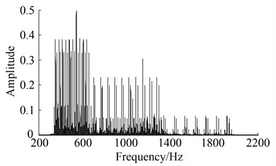
where and are the amplitude and the phase modulation parameter, respectively, and is the modulation frequency. In the Eqs. (9) and Eqs. (10), there are complex modulation sidebands in the spectrum of vibration signals of the gearbox transmission system. Thus, both the meshing frequency and the modulation frequencies vary with the rotation speed of the input shaft. The spectrum of the simulated signal is shown in Fig. 1(a) and the spectrum with varying modulation frequencies is shown in Fig. 1(b). The sampling frequency is 10 kHz and the sample time is 10 seconds, and speed ascends from 11 Hz to 20 Hz linearly in 10 seconds. As a result, it is very difficult to recognize meshing frequency and modulated frequencies in the spectrum.
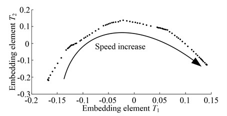
Although the time-frequency spectrum can be calculated, the feature dimension is too high (time × frequency) to extract effective features which can precisely depict the system conditions. To this end, the proposed method is used to reduce the high-dimensional features. The width of sliding window is set to 10000, the sliding step is 5000, and the spectrum is used as the original feature set. The two-dimensional embedding result obtained by KMML is shown in Fig. 2, where and are the first column and the second column of embedding coordinates set , respectively. It can be seen that the low-dimensional embedding of the simulated signals is a continuous nonlinear curve in varying rotation speed, and the shape and distribution of curve is decided by the speeds and loads. Then if the operation state of machine change (such as chipped tooth), the features of sampled signal is different from that of normal state in same operation condition, the corresponding embedding coordinates of samples of fault state also have a sudden change in that of normal state. That is to say a new embedded manifold is reformed for the fault state. Because of the different spatial distribution of two embedded manifolds, the operation states of machine can be recognized by the clustering algorithm, such as self-organized map, artificial neural network, etc.
Fig. 1Spectrum and its harmonics of simulation signal of gearbox
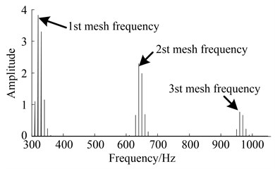
(a) Spectrum of simulation signal
(b) Spectrum with varying modulation frequencies
Fig. 2Low-dimensional embedding of the varying speeds
It is known that different gearbox faults also have different sidebands, decided by modulation parameters and . So in this paper, three kinds of modulation parameter are used to simulate different fault states, and the equations of waveform are defined as:
Then, the rotation speed is defined by where t changes in (0, 1). The simulated fault signals are shown in Fig. 3, where the sampling frequency is 3000 Hz, and noise is added into the signal. Each simulation signal is divided into 64 samples, whose sliding window width is 300, and the sliding step is 20. Then the samples are transformed into frequency domain, and the frequency spectra are divided into 20 equal bands. Thus the spectral energy on each band is calculated as the sum of the frequency amplitudes. Finally the 20 spectral energies are taken as the frequency-domain statistical features to characterize the simulation fault pattern. The number of training sets is 17 and the number of test sets is 4. The two-dimensional embedding extracted by LTSA and KMML algorithm is shown in Fig. 4, where the kernel function is . It can be seen that, compared with the result of LTSA, three embedded manifolds which have no overlaps between each other are extracted effectively by KMML. The test samples are used to classify by KNN. Due to the better separation capability of embedded manifolds, the test samples also are classified correctly.
Fig. 3The waveform of simulation fault
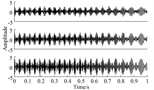
Fig. 4Embedded manifolds extracted by different learning algorithms
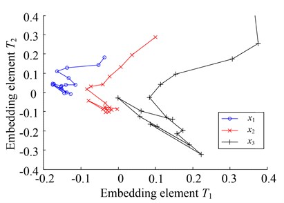
(a) KMML
(b) LTSA
5. Experimental applications of a gearbox system
5.1. Description of the simulator
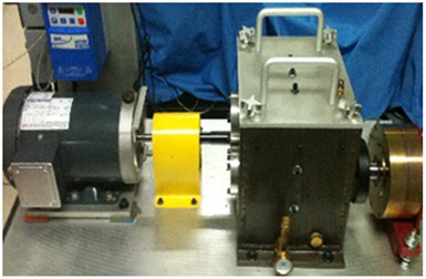
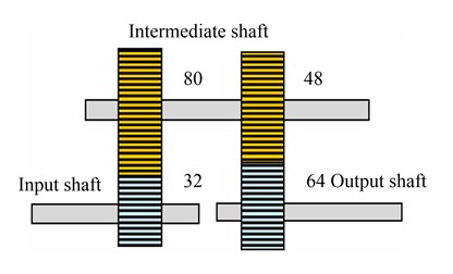
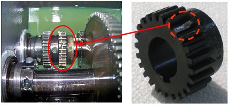
The experiments were conducted on Spectra Quest’s Gearbox Dynamics Simulator, as shown in Fig. 5(a). The objective is to relate the development of the feature component changes in varying operation conditions. The gearbox is driven by a 3 HP motor with a speed range of 0-4000 rpm. The speed inverter can be programmed, and the load provided by the brake was controlled by a current source. The modular design of the gearbox allows one to simulate various faults, either individually or jointly in a totally controlled environment. Fig. 5(b) illustrates a picture taken for the inside of the gearbox and a schematic of the two-stage parallel gearbox layout.
Two gears were tested in this study: (1) a health gear, (2) a large-chipped gear. The defected gears shown in Fig. 6 are the input gear (the 32-tooth one). For gear configuration, two operation conditions (varying load, varying load and speed simultaneously) were tested. For each test, accelerometer was mounted on the bearing seat. The vibration data was collected by a Noise & Vibration Analyzer – OR35, where the sampling frequency is 10 kHz.
Fig. 5Gearbox dynamics simulator
(a) Experiment table structure
(b) Two-stage parallel gear transmission
Fig. 6Faulted gears for the chipped tooth
5.2. The experiment of varying rotation speed
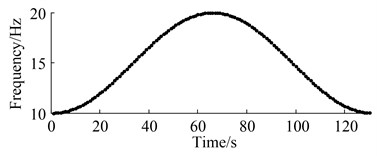
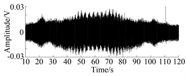
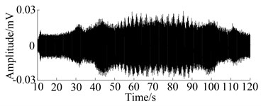
For the rotation speed of simulator, the cosine function is adopted as the model of varying speed which changes from 10 Hz to 20 Hz in 65 seconds. Therefore, the speed value per second is calculated according to the speed-time curve shown in Fig. 7, for the time resolution is 1 second and speed resolution is 0.1 Hz in the software of motor PC-control program. Finally, the rotation speed is programmed by the 65 discrete values of speed. Fig. 8 shows the waveform of the signal obtained from the gearbox in two states with varying rotation speed. It can obviously be seen that the amplitude of the waveform increases with the increase of rotation speed. However, the vibration level in Fig. 8(b) is the same as that in Fig. 8(a) with the effect of the varying speed.
Fig. 7Relationship of the speed and the time
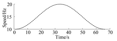
Fig. 8Waveform obtained from two operation states in varying speed
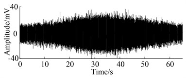
(a) Normal state
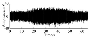
(b) Chipped tooth state
For such non-stationary signal, the time-frequency representation is shown in Fig. 9. However, it is difficult to visually identify the fault state from normal operating data. Thus in order to distinguish gearbox operation state, an appropriate dimension reduction tool is needed to extract the low-dimensional embedding.
Fig. 9Time-frequency representation of the signal in two operation states
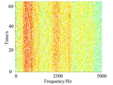
(a) Normal state
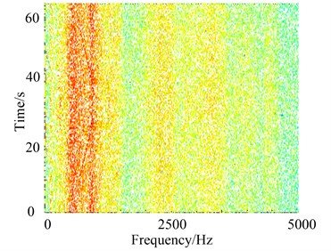
(b) Chipped tooth state
The vibration data is divided by slide Hanning window whose window width is 10000, and the degree of overlapping is 50 % (to ensure the continuous samples). Thus the set of training data consisting of 119 samples is constructed for each state (normal and chipped). The frequency spectra are divided into 20 equal bands, and then the 20 spectral energy features are taken as the statistical features to characterize the running state pattern.
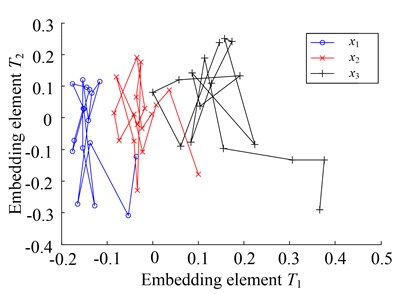
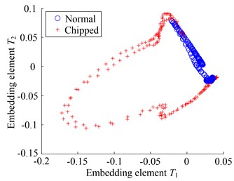
By the influence of the rotation speed, the Pseudo degree of freedom also increases. Therefore, in order to visually identify the fault, the intrinsic dimension is set to 2. The low-dimensional embedding results obtained by LTSA and KMML are compared, where the kernel function is gauss function with variance 0.01. Fig. 10(a) shows the two-dimensional representation of normal and chipped states. It embraces an overlap around the higher speeds. This may results in false diagnosis in the visual coordinate space. The main reason is that, in the higher speeds, the features of frequency band energy of chipped tooth are similar to that in the normal state, thus due to the influence of space reduction, the feature set of the two operation states can emerge overlap partly.
Fig. 10Two-dimensional representation for different learning algorithm
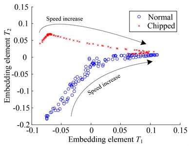
(a) LTSA
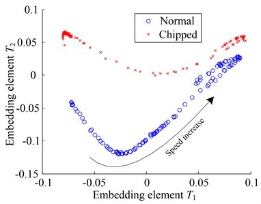
(b) KMML
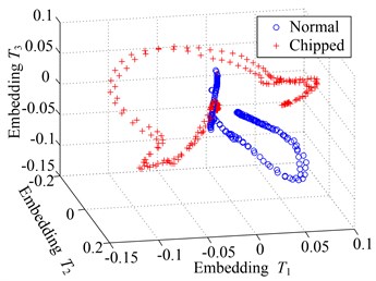
Fig. 10(b) shows the two-dimensional representation of the feature set obtained by KMML method. It can obviously be seen that the embedded manifold coordinate has a significant difference between normal and chipped-tooth states. Due to kernel mapping, the class separability can be enhanced. Even though the embedding value increase with the rotation speed increases in embedding element coordinate direction, the embedded manifold of the two running conditions also has no overlaps. It is very convenient to identify the fault pattern in the varying speed condition. Finally, the 33 test samples are classified correctly.
5.3. The experiment of variable rotating speed and load
As discussed above, the proposed method is an effective classification for varying speed. However, in practice, except for the varying speed, load of gearbox system also changes by the influence of many factors, such as non-uniformity in material which can result in the load fluctuation of spindle. Then the speed increase can result in the amplitudes increasing of features. So it is difficult to identify this content as loading-related or fault-related. Therefore further experiments with varying loads need to be done.
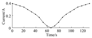
In the process of varying speeds and loads, loading force is controlled by a current source using the magnetic brake. Fig. 11 shows the varying curve of rotation speed and load. It can be seen that the current values of load force change from 0 A to 40 A in 130 seconds, where it is large in slow speeds and vice versa. Fig. 12 shows the waveform of the signal obtained from the two running states, where sampling frequency is 6400 Hz. Each plot depicts the changes of waveform in varying speed and load condition. It can obviously be seen that the amplitude of vibration waveform increases with the increase of rotation speed. The vibration level in Fig. 12(b) is also the same as that in Fig. 12(a).
Fig. 11Relationship between speed-time and current-time
(a) Speed curve
(b) Current curve
Fig. 12Waveform of signals obtained from two operation states in varying speeds and loads
(a) Normal state
(b) Chipped tooth state
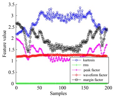
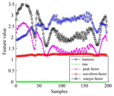
It should be noted that classic diagnostic features usually depend on the value of the external load. Fig. 13 shows the diagnostic features [16] (standard deviation, kurtosis, root mean square, absolute mean, peak factor, waveform factor, and margin factor) of 200 samples of varying speeds and loads in two operating states. The vibration level of each variable in normal (in Fig. 13(a)) is compared with that of chipped fault (in Fig. 13(b)). It was clear that considering the vibration level of the variable itself, the fault pattern cannot be detected or identified.
Considering the effect of speed and load, the vibration data is divided by sliding window, where the window width is 6400, and degree of overlapping 50 % is used. The analysis sample number for each operation state is set to 240, and then each sample is transformed by the 'db3' wavelet which the scale 1, 2, …, 20. Thus in the discrete 20 scales, the features of sample are calculated as the sum of absolute of the wavelet coefficients and mathematically is defined by where are wavelet coefficients. After that, a total of 480 samples including two states were considered for the 20 features, thus the high-dimensional feature space , where 480 and 20.
Fig. 13Feature value obtained from two operation states in varying speeds and loads
(a) Normal state
(b) Chipped tooth state
The two-dimensional representation of the feature set obtained by KMML is shown in Fig. 14(a). It can obviously be seen that, due to increasing the degree of freedom of embedding in the condition of varying speed and load, the embedded manifolds captured by KMML form two operation states have a larger overlap. This means that it is difficult to have a good recognition effect. Therefore, the three-dimensional embedded manifold is also extracted and shown in Fig. 14(b). It is very convenient to identify that the overlap of two embedding distribution is much lower. The 20 test samples are adopted to be classified and the classification error is only 5 %.
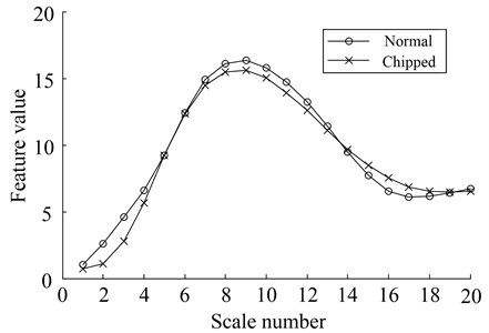
Obviously, in embedding space, the misjudgment of two states only occurs at overlapping region for the similar the embedding coordinates, such as the samples of normal and chipped in 11.9 Hz speed. The corresponding original 20-dimensional features are shown in Fig. 15. The number 1, 2, …, 20 of the horizontal axis in the graph respectively stands for different scales, and vertical axis is the feature value under scales. It is found that the feature values under normal and chipped states are almost the same representation. Therefore, in the condition of varying speed and load, except for the samples in overlapping region, other samples can be classified correctly for the larger different of embedding coordinates.
Fig. 14Representation for varying operation conditions with different embedding spaces
(a) Two-dimensional embedding
(b) Three-dimensional embedding
Fig. 15Frequency domain feature in the condition of speed is 11.9 Hz
6. Conclusions
In this paper, a new method of kernel mapping manifold learning for fault detection is proposed. Considering the varying operation condition, the kernel mapping is introduced to improve the identification of embedded manifold coordinates which accurately captures the differences of varying operation conditions.
The proposed method is applied to gearbox simulation and practical data sets collected by varying speeds and loads in the interest of exploratory data analysis and visualization. In these experiments, the method can discover the low-dimensional spaces and revealed the interesting and separability of data patterns that are not accessible by LTSA.
It should be noted that existing manifold learning approaches already proposed in literatures also use LTSA, ISOMAP, LLE for data reduction, but they are not suitable to analyze varying operation conditions. It should be added that just a few works may be found in the context of mechanical drives, time varying loads and non-stationary conditions. So it is believed that the data processing method proposed here may be useful for scientists and engineers in condition monitoring and fault diagnosis.
References
-
Kusiak A., Li W. Y. The prediction and diagnosis of wind turbine faults. Renewable Energy, Vol. 36, Issue 1, 2011, p. 16-23.
-
Combet F., Zimroz R. A new method for the estimation of the instantaneous speed relative fluctuation in a vibration signal based on the short time scale transform. Mechanical Systems and Signal Processing, Vol. 23, Issue 4, 2009, p. 1382-1397.
-
Baydar N., Chen Q., Ball A., Kruger U. Detection of incipient tooth defect in helical gears using multivariate statistics. Mechanical Systems and Signal Processing, Vol. 15, Issue 2, 2001, p. 303-321.
-
Li F. C., Meng G., Ye L., Chen P. Wavelet transform-based higher-order statistics for fault diagnosis in rolling element bearings. Journal of Vibration and Control, Vol. 14, Issue 11, 2008, p. 1691-1709.
-
Wu J. D., Chiang P. H. Application of Wigner-Ville distribution and probability neural network for scooter engine fault diagnosis. Expert Systems with Applications, Vol. 36, Issue 2, 2009, p. 2187-2199.
-
Chandran P., Lokesha M., Majumder M.C., Raheem K. F. Application of Laplace wavelet kurtosis and wavelet statistical parameters for gear fault diagnosis. International Journal of Multidisciplinary Sciences and Engineering, Vol. 3, Issue 9, 2012, p. 1-7.
-
Malhi A., Gao R. X. PCA-based feature selection scheme for machine defect classification. IEEE Transactions on Instrumentation and Measurement, Vol. 53, Issue 6, 2004, p. 1517-1525.
-
Trendafilova I., Cartmell M., Ostachowicz W. Vibration based damage detection in an aircraft wing scaled model using principal component analysis and pattern recognition. Journal of Sound Vibration, Vol. 313, Issue 3, 2008, p. 560-566.
-
Yoon S., MacGregor J. F. Fault diagnosis with multivariate statistical models, Part I: Using steady state fault signatures. Journal of Process Control, Vol. 11, Issue 4, 2001, p. 387-400.
-
Villa L. F., Renones A., Peran J. R., DeMiguel L. J. Statistical fault diagnosis based on vibration analysis for gear test-bench under non-stationary conditions of speed and load. Mechanical Systems and Signal Processing, Vol. 29, Issue 2, 2010, p. 436-446.
-
Tenenbaum J., Silva D. D., Langford J. A global geometric framework for nonlinear dimensionality reduction. Science, Vol. 290, Issue 5500, 2000, p. 2319-2323.
-
Roweis S., Saul L. Nonlinear dimensionality reduction by locally linear embedding. Science, Vol. 290, Issue 5500, 2000, p. 2323-2326.
-
Belkin M., Niyogi P. Laplacian eigenmaps for dimensionality reduction and data representation. Neural Computation, Vol. 15, Issue 6, 2003, p. 1373-1396.
-
Zhang Z. Y., Zhang H. Y. Principal manifolds and nonlinear dimensionality reduction via tangent space alignment. SIAM Journal of Scientific Computing, Vol. 26, Issue 1, 2005, p. 313-318.
-
Yang J. H., Xu J. W., Yang D. B. Noise reduction method for nonlinear time series based on principal manifold learning and its application to fault diagnosis. Chinese Journal of Mechanical Engineering, Vol. 42, Issue 8, 2006, p. 154-158.
-
Jiang Q. S., Jia M. P., Hu J. Z. Machinery fault diagnosis using supervised manifold learning. Mechanical Systems and Signal Processing, Vol. 23, Issue 7, 2009, p. 2301-2311.
-
Li M. L., Liang L., Wang S. A. Mechanical impact feature extraction method based on nonlinear manifold learning of continuous wavelet coefficient. Journal of Vibration and Shock, Vol. 31, Issue 1, 2012, p. 106-111.
-
Bartelmus W., Zimroz R. A new feature for monitoring the condition of gearboxes in nonstationary operating systems. Mechanical Systems and Signal Processing, Vol. 23, Issue 5, 2009, p. 1528-1534.
About this article

This work was supported by National Natural Science Foundation of China (No. 51075323).
