Finite element model updating using base excitation response function

Fei, Qingguo; Jiang, Dong; Zhang, Dahai; Han, Xiaolin

Journal of Vibroengineering

Browse Journal

Submit article

Published: 31 March 2013

Check for updates

Finite element model updating using base excitation response function

Qingguo Fei¹

Dong Jiang²

Dahai Zhang³

Xiaolin Han⁴

^{1, 2, 3, 4}Department of Engineering Mechanics, Southeast University, Nanjing 210096, China

^{1, 2, 3, 4}Jiangsu Key Laboratory of Engineering Mechanics, Nanjing 210096, China

Cite the article Download PDF

Downloads 1628

Abstract

Finite element model updating is an effective way to build accurate analytical models for structures. Most of the available updating methods employ information from modal testing. However, in astronautics engineering, information provided by vibration table testing is more valuable than those from modal testing. Therefore, it is necessary to study updating methods which can adopt information from vibration table testing. This paper presents the study on such issue. The base excitation response function is analyzed with the assumption that the vibration table gives the structure a single direction motion excitation. Model updating method which adopts the response function is then proposed. In the numerical simulation, several case studies are constructed for a truss structure with small or significant modeling errors respectively. Data selection, which has great influence on the success of updating, is carefully studied. A novel adaptive data selection approach is suggested. Simulation results show that model updating converge with good accuracy when the adaptive data selection approach is used.

1. Introduction

Finite element modeling plays a key role in structural design and analysis. However, there are three commonly encountered forms of errors which give rise to modeling inaccuracy [1]: model structure error, model parameter error and model order error. Hence, model updating need to be performed to improve the quality of finite element models (FEM) so that the models could be applied with confidence.

In the past decades, extensive researches have been carried out on model updating. Varieties of model updating methods have been proposed [2]. Relevant key issues, such as sensitivity analysis [3], regularization techniques [4-5], estimation techniques [6-8], model evaluation [9], etc., have been deeply studied until recently. These efforts make great contribution to model updating and make it more and more practical. In fact, several successful applications on complex engineering structures could be seen from the literatures [10-13].

However most of the dynamic model updating methods employ modal information, including modal frequencies and mode shapes. Several employ frequency response function (FRF) [14], which is actually transfer function between structural motion and force excitation. This is reasonable since the modal properties are inherent properties of structures and the accuracy of modal parameters and frequency response functions could be assured in certain extent by the rapid development of dynamic testing equipment and modal identification methods. However, modal testing is not always necessary in astronautics engineering.

Comparing with modal testing, vibration table testing is much more important in astronautics engineering and is an essential testing to be carried out on astronautics structures for two reasons: (1) In the launching stage, the astronautics structures are excited by inertia forces. To make sure that the structures are safe in that stage, vibration table testing is an essential and the only approach to simulate the load on structures during launching. Meanwhile, excitation forces could only be added to limited numbers of points of structures in the modal testing. (2) The preparation of modal testing is time-consuming, e.g., selection of sensor location, selection of excitation points. This is not always acceptable. In practice, modal testing is performed only for new type of satellite platform while vibration table testing need to be performed for every single astronautics structure.

To circumvent that problem, some researchers proposed to identify modal parameters from vibration table testing data so that the updating methods based on modal parameters could be used to update the FEM of structures under base excitation [15]. However, discussions on the advantages and disadvantages of modal parameters and frequency response functions give us some conclusions: (1) Frequency response function contains more and fidelity information than modal parameters. (2) Mode shape pairing could be avoided when using frequency response function. These conclusions tell us that it’s a better choice to use vibration table testing data rather than to identify modal parameters from the data. Therefore, it is necessary to study updating methods which can adopt vibration table testing data, or more specifically, the base excitation response function.

This paper presents the study on model updating using base excitation response function (BERF). The paper is organized as follows: In Section 2, base excitation response function is analyzed with the assumption that the vibration table gives the structure a single direction motion excitation. In Section 3, model updating method which adopts the base excitation response function is proposed. In Section 4 to Section 6, four case studies are constructed in the simulation study for a truss structure with small and significant modeling errors to verify the proposed method and to study data selection problem.

2. Base excitation response function

As mentioned above, frequency response function is actually the transfer function between structural motion and force excitation (motion-to-force). For vibration table testing, structures are excited by base movement. The base excitation response function is the transfer function between structural motion and base motion excitation (motion-to-motion). Suppose the vibration table gives the structure a single direction motion excitation, the base excitation response function could be calculated as follows:

1

\ddot{Y} (ω) = H_{m} (ω) A_{0} (ω),

where $A_{0} (ω)$ is the base movement acceleration, $\ddot{Y} (ω)$ is the absolute acceleration of the structure, $H_{m} (ω)$ is the base excitation response function.

$\ddot{Y} (ω)$ could be described as:

2

\ddot{Y} (ω) = {\ddot{V}}_{0} (ω) + \ddot{V} (ω),

where $\ddot{V} (ω)$ represents the acceleration of structural elastic motion with respect to the base, ${\ddot{V}}_{0} (ω)$ represents the acceleration of structural rigid motion and could be defined as:

3

{\ddot{V}}_{0} (ω) = A_{0} (ω) Σ,

where $Σ$ is the inertia force distribution vector, the element of the vector could be 1 or 0.

The structural elastic motion is governed by the following equation:

4

M \ddot{v} + C \dot{v} + K v = {- a}_{0} M Σ,

where $M$ , $C$ and $K$ are the structural mass matrices, damping matrices and stiffness matrices.

The Fourier transform of Eq. (4) is:

5

\ddot{V} (ω) = - A_{0} (ω) H_{A} (ω) M Σ,

where $H_{A} (ω)$ is the frequency response function (motion-to-force) and defined as:

6

H_{A} (ω) = \frac{- ω^{2}}{- ω^{2} M + j ω C + K} .

Replace $\ddot{V} (ω)$ and ${\ddot{V}}_{0} (ω)$ in Eq. (2) with Eq. (3) and Eq. (5):

7

\ddot{Y} (ω) = - A_{0} (ω) H_{A} (ω) M Σ + A_{0} (ω) Σ = [I - H_{A} (ω) M] Σ A_{0} (ω) .

Comparing Eq. (7) with Eq. (1), base excitation response function is:

8

H_{m} (ω) = [I - H_{A} (ω) M] Σ .

3. Model updating using base excitation response function

3.1. Sensitivity base finite element model updating

Suppose $p_{0}$ represents the structural parameter of the initial FEM. Let $f$ represents structural characteristics. These structural characteristics could be modal parameter, or frequency response function or base excitation response function in this study. Obviously $f$ is function with respect to $p_{0}$ . The Taylor expansion of $f$ is:

9

f (p) ≅ f (p_{0}) + \sum_{n = 1}^{n_{p}} \frac{\partial f}{\partial p_{n}} Δ p_{n} .

Rewritten Eq. (9) into matrix form:

10

S \{Δ p\} ≅ Δ f,

where $Δ f$ is the residue vector, $Δ p$ is the modification vector for structural parameters, $S$ is the sensitivity matrix:

11

Δ f = \{f (p)\} - \{f (p_{0})\},

12

Δ p = {(Δ p_{1}, Δ p_{2}, \dots, Δ p_{n_{p}})}^{T},

13

S = [\begin{matrix} \frac{\partial f_{1}}{\partial p_{1}} & \dots & \frac{\partial f_{1}}{\partial p_{n_{p}}} \\ ⋮ & ⋱ & ⋮ \\ \frac{\partial f_{n_{f}}}{\partial p_{1}} & \dots & \frac{\partial f_{n_{f}}}{\partial p_{n_{p}}} \end{matrix}],

where $n_{p}$ is the number of structural parameters to be updated, $n_{f}$ is the number of structural characteristics used in the updating. In this study, structural characteristics $f$ are used in the base excitation response function. The sensitivity analysis of the base excitation response function is given below.

3.2. Sensitivity analysis of base excitation response function

According to Eq. (8), sensitivity of the base excitation response function with respect to structural parameter $p$ is:

14

\frac{\partial H_{m}}{\partial p} = - [\frac{\partial H_{A}}{\partial p} M + H_{A} \frac{\partial M}{\partial p}] Σ,

where $\frac{\partial H_{A}}{\partial p}$ is:

15

\frac{\partial H_{A}}{\partial p} = - H_{A} \frac{\partial H_{A}^{- 1}}{\partial p} H_{A},

where $H_{A}$ is the frequency response function as those in Eq. (5).

4. Numerical simulation: six parameters with small modeling error

4.1. GARTEUR truss structure

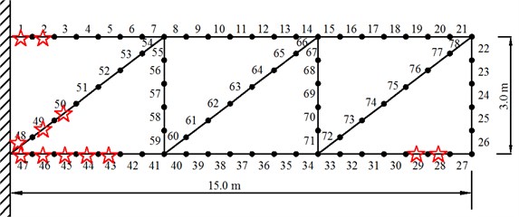
The proposed method is applied in the model updating of a GARTEUR truss structure shown in Fig. 1. The GARTEUR structure has two points fixed to the base. The FEM of the GARTEUR structure consists of 36 2-D beam elements. Each beam segment is a superposition of an axial bar element and a bending beam element. Each node of the beam element has three DOFs (two translations and one rotation) and hence, the total number of DOFs in the FEM is 90. Following material properties are used for the initial model: Young’s modulus is assumed to be 7.5×10¹⁰·N/m² and density 2800 kg/m³. For the bar element, the cross-sectional areas are $0.004 m^{2}$ . For the bending beam elements, the second moment of area is assumed to be the same for all the elements and is assumed to be 0.0756 m⁴.

Fig. 1The GARTEUR structure

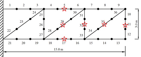
In order to generate the simulated experimental data, stiffness modeling deviations are introduced in the elements of the analytical model by modifying Young’s modulus of six elements as shown in Table 1. These elements are marks with stars in Fig. 1. Two simulated experimental cases are simulated as listed in Table 1. Assuming that the base gives the structure vertical motion excitation, and all the translational dimensions of freedom are measurable.

Table 1Parameter values for initial model and simulated experimental cases

Element No.	5	11	17	29	32	35
Young’s modulus: Initial model $(10^{10} N / m^{2})$	7.5	7.5	7.5	7.5	7.5	7.5
Young’s modulus: Case 1 $(10^{10} N / m^{2})$	6.75	6.75	6.75	6.75	6.75	6.75
Young’s modulus: Case 2 $(10^{10} N / m^{2})$	6	6	6	6	6	6

In the study of model updating using FRF, a key problem is how to select the data. Although the most common rule is to select the data close to the peaks of the experimental frequency response functions (‘close-to-peak’ rule), this problem will be further discussed in the study of model updating using BERF in the following chapters.

4.2. Case 1: data selection and model updating

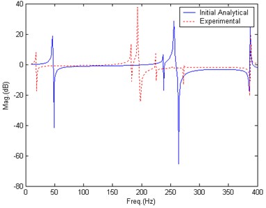
Fig. 2 gives the comparing of analytical BERF and the simulated experimental BERF. It could be seen from Fig. 2 that peaks of the analytical BERF and the simulated experimental BERF in the frequency band from 200 Hz to 400 Hz are different.

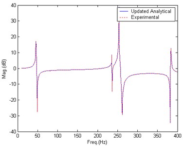
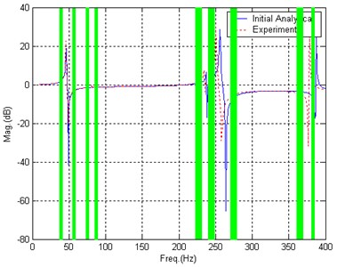
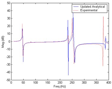
Data in nine frequency bands close to the peaks of simulated experimental BERF are used during the updating. The nine frequency bands are marked with bars as shown in Fig. 3. After 20 iterations, the updating converges to satisfactory results. Fig. 4 gives the comparison of BERF after updating. Table 2 lists the updated value of parameters.

Fig. 2Comparison of BERF, before updating, Case 1

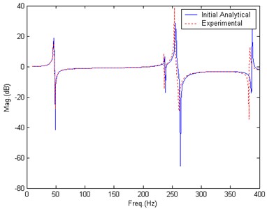
Fig. 3Data selection, Case 1

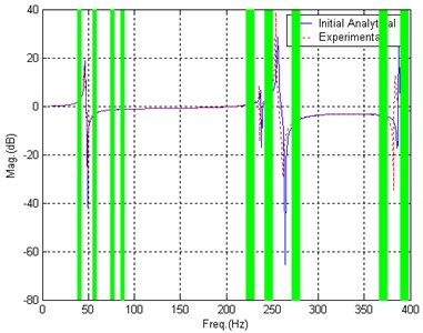
Table 2Updated results, Case 1

Element No.	5	11	17	29	32	35
Updated results: Case 1 (10¹⁰·N/m²)	6.75	6.75	6.75	6.75	6.75	6.75

Fig. 4Comparison of BERF, after updating, Case 1

4.3. Case 2: data selection and model updating

In this case, modeling errors are more significant than those of Case 1. Data selection approach is firstly the same as that in Case 1 (‘close-to-peak’ rule) and data in nine frequency bands are used in the updating. The data are marked with bar as demonstrated in Fig. 5.

Fig. 5Data selection, Case 2

However, the updating doesn’t converge as expected after 30 iterations. Fig. 6 shows the comparison of BERF after 30 iterations. It could be found that the differences between peaks of analytical BERF and experimental BERF seem not to be decreased. It is also found that the values of structural parameters are not converging in the updating.

Fig. 6Comparison of BERF, after updating, Case 2

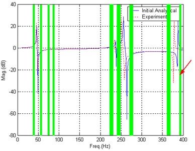
From the updating result, it could be concluded that the ‘close-to-peak’ data selection rule need to be adjusted. The new data selection is shown in Fig. 7. Comparing with Fig. 5, it could be found that the only difference is the ninth frequency band is moved a little bit right as marked by the arrow in Fig. 7.

Fig. 7New data selection, Case 2

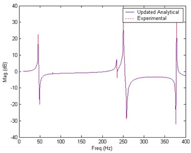
This adjustment works. After 20 iterations, the updating converges to satisfactory results. Fig. 8 gives the comparison of BERF after updating. Table 3 lists the updated parameters’ value.

Table 3Updated results, Case 2

Element No.	5	11	17	29	32	35
Updated results: Case 2 (10¹⁰·N/m²)	6	6	6	6	6	6

Fig. 8Comparison of BERF, after new updating, Case 2

4.4. Discussion on data selection

The only difference between Fig. 5 and Fig. 7 is the ninth frequency band. If we take a careful look at the ninth frequency band in Fig. 5, it could be seen that the band locates between one experimental BERF peak and one analytical BERF peak. This analytical BERF peak will move left and move closer to the experimental BERF peak in the updating process, and will pass the ninth frequency band. Meanwhile, if we take a look at ninth frequency band in Fig. 7, it could be seen that the band locates right to the analytical BERF peak. In the updating process, the analytical BERF peak will not pass the ninth frequency band. Furthermore, if we take a look at other eight frequency bands (same for Fig. 5 and Fig. 7), it could be found that none of them will be passed by the analytical BERF peak during the updating.

According to such analyses, two data selection rule including ‘close-to-peak’ rule could be suggested below:

(1) Data in the frequency bands close to the peak of experimental BERF are prior choices (‘close-to-peak’ rule),

(2) Frequency bands which will be passed by the analytical peaks in the updating process should not be selected.

5. Numerical simulation: six parameters with significant modeling error

5.1. Simulated modeling error

The GARTEUR structure in 3.1 is used again. Young’s moduli of six elements are assumed to have modeling errors. Modeling error is significant as shown in Table 4. From Fig. 9, the differences between analytical and experimental peaks are significant.

Table 4Parameter values for initial model and simulated experimental Case 3

Element No.	5	11	17	29	32	35
Young’s modulus: Initial model (10¹⁰·N/m²)	7.5	7.5	7.5	7.5	7.5	7.5
Young’s modulus: Case 3 (10¹⁰·N/m²)	0.75	0.75	0.75	0.75	0.75	0.75

Fig. 9Comparison of BERF, before updating, Case 3

5.2. Case 3: data selection and model updating

According to the rules in section 4.4, data in three frequency bands below 200 Hz satisfy the two rules and are included in the beginning of updating. Data in five frequency bands beyond 200 Hz only satisfy ‘close-to-peak’ rule and are not included in the updating. These eight frequency bands are marks with bars as shown in Fig. 10.

Fig. 11 gives the comparison of BERF after 40 iterations. It could be seen that the difference between analytical BERF and experimental become much smaller. There are four frequency bands of data satisfy the two rules. The second band move left with the first analytical peak and getting closer to the first experimental peak.

Fig. 10Data selection at the beginning of updating, Case 3

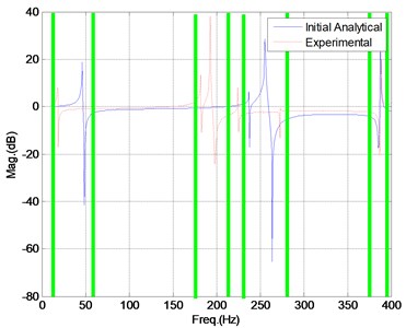
Fig. 11Data selection after 40 iterations, Case 3

After 70 iterations, the updating converges to satisfactory results. Fig. 12 gives the comparison of BERF after updating. Table 5 lists the updated value of parameters.

Table 5Updated results, Case 3

Element No.	5	11	17	29	32	35
Updated results: Case 3 (10¹⁰·N/m²)	0.75	0.75	0.75	0.75	0.75	0.75

Fig. 12Comparison of BERF, after updating, Case 3

5.3. Adaptive data selection

According to the case studies, an adaptive data selection approach with three rules could be suggested below:

(1) Data in the frequency band close to the peak of experimental BERF are prior choices,

(2) Frequency bands which will be passed by the analytical peaks in the updating process should not be selected,

(3) Select data in frequency bands which satisfy the above two rules at the beginning of updating; supplement those data which doesn’t satisfy the two rules at the beginning but become satisfying the above two rules during the updating process.

6. Numerical simulation: twelve parameters with significant modeling error

6.1. Simulated modeling error

The new GARTEUR structure used here (Fig. 13) has similar geometry to that of section 4.1. But the FEM is more complex. It consists of 78 2-D beam elements and 222 DOFs. Material properties used for the initial model are: Young’s modulus is 7.5×10¹⁰·N/m², material density is 2800 kg/m³. Cross-sectional areas is 0.004 m², 0.006 m² and 0.003 m² for the horizontal bar element, the vertical bar element and the diagonal bar element respectively. For the bending beam elements, the second moment of area is assumed to be the same for all the elements and is assumed to be 0.0756 m⁴. Young’s moduli of twelve elements are assumed to have modeling errors as listed in Table 6. Twelve elements are marked with stars in Fig. 13.

Table 6Paramter values for initial model and simulated experimental Case 4

Element No.	1	2	28	29	43	44
Young’s modulus: Initial model (10¹⁰·N/m²)	7.5	7.5	7.5	7.5	7.5	7.5
Young’s modulus: Case 4 (10¹⁰·N/m²)	0.75	0.75	15	15	15	15
Element No.	45	46	47	48	49	50
Young’s modulus: Initial model (10¹⁰·N/m²)	7.5	7.5	7.5	7.5	7.5	7.5
Young’s modulus: Case 4 (10¹⁰·N/m²)	8.25	0.75	0.75	0.75	0.75	0.75

Fig. 13The new GARTEUR structure FEM

6.2. Case 4: data selection and model updating

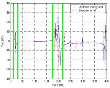
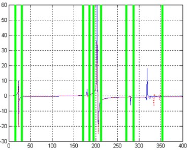
It could be seen from Fig. 14 that the experimental BERF is much different from analytical BERF. According to the adaptive data selection, data in three frequency bands below 200 Hz should be included in the beginning of updating as shown in Fig. 15.

Fig. 16 gives the comparison of BERF after 100 iterations. It could be seen that the difference between analytical BERF and experimental become smaller than the beginning. There are now nine frequency bands of data satisfy the two rules.

Fig. 14Comparison of BERF, before updating, Case 4

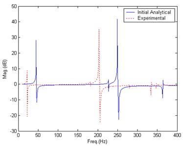
Fig. 15Data selection at the beginning of updating, Case 4

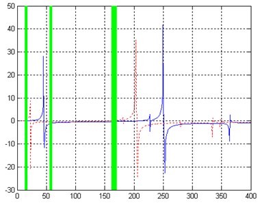
Fig. 16Data selection after 100 iterations, Case 4

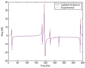
After nearly 300 iterations, the updating converges to satisfactory results. Fig. 17 gives the comparison of BERF after updating. Table 7 lists the updated value of parameters.

Fig. 17Comparison of BERF, after updating, Case 4

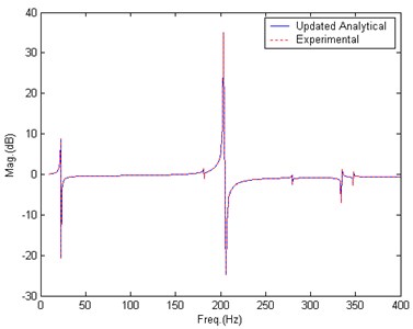
Table 7Updated results, Case 4

Element No.	1	2	28	29	43	44
Updated result: Case 4 (10¹⁰·N/m²)	0.75	0.75	15	15	15	15
Element No.	45	46	47	48	49	50
Updated result: Case 4 (10¹⁰·N/m²)	8.25	0.75	0.75	0.75	0.75	0.75

7. Conclusions

Considering the importance of vibration table testing in astronautics engineering, finite element model updating using base excitation response function is studied in this paper. The BERF is defined as the transfer function between structural motion and base motion excitation. The function is analyzed as the combination of two accelerations: structural elastic motion acceleration with respect to the base and structural rigid motion acceleration. Model updating method which adopts the function is proposed based on that analysis. Four case studies are constructed in the simulation study for a truss structure with different small and significant modeling errors to verify the proposed method and to study data selection problem. A novel data selection approach is proposed with three rules: (1) Data in the frequency band close to the peak of experimental BERF are prior choices, (2) Frequency bands which will be passed by the analytical peaks in the updating process should not be selected, (3) Select data in frequency bands which satisfy the above two rules at the beginning of updating; supplement those data which doesn’t satisfy the two rules at the beginning but become satisfying the two rules during the updating process.

References

M. I. Friswell, J. E. Mottershead. Finite element model updating in structural dynamics. Kluwer Academic Publishers, Dordrecht, 1995.

Search CrossRef
J. E. Mottershead, M. Link, M. I. Friswell. The sensitivity method in finite element model updating: a tutorial. Mechanical Systems and Signal Processing, Vol. 25, Issue 7, 2011, p. 2275-2296.

Search CrossRef
Z. R. Lu, S. S.Law. Features of dynamic response sensitivity and its application in damage detection. Journal of Sound and Vibration, Vol. 303, 2007, p. 503-524.

Search CrossRef
B. Titurus, M. I. Friswell. Regularization in model updating. International Journal for Numerical Methods in Engineering, Vol. 75, Issue 4, 2008, p. 440-478.

Search CrossRef
B. Weber, P. Paultre, J. Proulx. Consistent regularization of nonlinear model updating for damage identification. Mechanical Systems and Signal Processing, Vol. 23, Issue 6, 2009, p. 1965-1985.

Search CrossRef
X. G. Hua, Y. Q. Ni, Z. Q. Chen, J. M. Ko. An improved perturbation method for stochastic finite element model updating. International Journal for Numerical Methods in Engineering, Vol. 73, 2008, p. 1845-1864.

Search CrossRef
H. Haddad Khodaparast, J. E. Mottershead, M. I. Friswell. Perturbation methods for the estimation of parameter variability in stochastic model updating. Mechanical Systems and Signal Processing, Vol. 22, Issue 8, 2008, p. 1751-1773.

Search CrossRef
C. Soize, E. Capiez-Lernout, R. Ohayan. Robust updating of uncertain computational models using experimental modal analysis. AIAA Journal, Vol. 46, Issue 11, 2008, p. 2955-2965.

Search CrossRef
Qingguo Fei, Jifeng Ding, Xiaolin Han, Dong Jiang. Criterion of evaluating initial model for effective dynamic model updating. Journal of Vibroengineering, Vol. 14, Issue 3, 2012, p. 1362-1369.

Search CrossRef
Dennis Goge. Automatic updating of large aircraft models using experimental data from ground vibration testing. Aerospace Science and Technology, Vol. 7, Issue 1, 2003, p. 33-45.

Search CrossRef
Qingguo Fei, Youlin Xu, Chilun Ng et al. Structural health monitoring oriented finite element model of Tsing Ma Bridge tower. International Journal of Structural Stability and Dynamics, Vol. 7, Issue 4, 2007, p. 647-668.

Search CrossRef
H. Shahverdi, C. Mares, W. Wang, J. E. Mottershead. Clustering of parameter sensitivities: examples from a helicopter airframe model updating exercise. Shock and Vibration, Vol. 16, Issue 1, 2009, p. 75-88.

Search CrossRef
Bijaya Jaishi, Weixin Ren. Structural finite element model updating using ambient vibration test results. Journal of Structural Engineering, Vol. 131, Issue 4, 2005, p. 617-628.

Search CrossRef
D. Celic, M. Boltezar. Identification of the dynamic properties of joints using frequency-response functions. Journal of Sound and Vibration, Vol. 317, Issue 1-2, 2008, p. 158-174.

Search CrossRef
J. G. Beliveau, F. R. Vigneron, Y. Soucy, S. Draisey. Modal parameter estimation from base excitation. Journal of Sound and Vibration, Vol. 107, Issue 3, 1986, p. 435-449.

Search CrossRef

About this article

Received

30 October 2012

Accepted

28 February 2013

Published

31 March 2013

Keywords

finite element model updating

base excitation response function

adaptive data selection

numerical simulation

Acknowledgements

The authors of the paper would like to express appreciation of the support from National Natural Science Foundation of China (10902024), Ministry of Education Program for New Century Excellent Talents in University (NCET-11-0086), Jiangsu Natural Science Foundation (BK2010397), and Foundation for Distinguished Young Teacher of Southeast University.

This is an open access article distributed under the Creative Commons Attribution License, which permits unrestricted use, distribution, and reproduction in any medium, provided the original work is properly cited.