Modal parameter identification and finite element model updating of a long-span aqueduct structure based on ambient excitation

2.1. Arrangement of monitoring points

The studied aqueduct, located in Tiantai County, Zhejiang, is divided into 5 spans. Each span is 36 m long. The main arch ring is circular arc, and the center angle is 116°32'. The length of the inlet and outlet section is about 19 m, and the maximum height from the top of the trench to the riverbed is 21.5 m. The aqueduct body is 5.24 m wide and 3.5 m high, the sidewalks on both sides of the bank are 0.8 m wide, and the trapezoid cross section has a design flow of 12.2 m³/s. The main materials include: 50^# masonry block stone groove body, 100^# masonry strip stone arch ring, 50^# masonry block stone arch abdomen, 80^# masonry strip stone pier surface, 75^# masonry block stone pier body, 150^# concrete pier cap, and 200^# sidewalk frame on the top of the groove on the right bank. The pier is poured by underwater concrete with pipe piles of grab hammer. The depth of the column is 12 m, and the bottom of the pile is deep into the bedrock. There are 4 pile foundations for each pier foundation. Fig. 1 shows the profile of the aqueduct.

Fig. 1An actual aqueduct in China

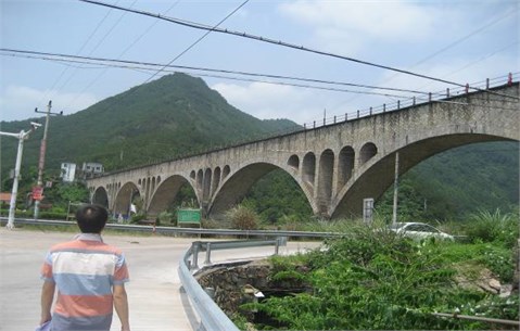
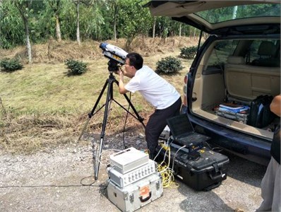
Fig. 2 shows eight horizontal vibration measuring points arranged on the top of the left half of aqueduct according to the general vibration law of aqueduct structure. The sensor used for base point vibration test is the 941B vibration pickup produced by the Institute of engineering mechanics, China Earthquake Administration. The other seven vibration measuring points are measured by scanning with PSV-500 laser vibrometer produced by German Polytec company. This test method reduces the wiring and improves the test efficiency and accuracy. The vibration signal is connected to DH5920 dynamic data acquisition system through 941 special amplifier for acquisition. Fig. 3 shows the test site.

Fig. 2Arrangement of aqueduct vibration measuring points

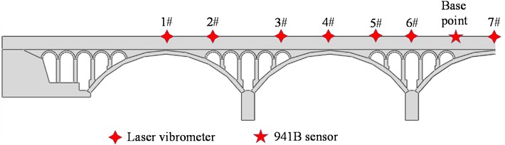
Fig. 3Laser scanning vibration measurement site

2.2. Modal test results

Since the input of aqueduct structure is inconvenient to measure in practical application, the identification of natural frequency is often based on the auto power spectrum of structural response. However, due to the interference of measurement noise and excitation spectrum, the peak value of structure auto power spectrum is not necessarily the modal frequency. According to the following principles, the structural modal frequency can be determined by the difference of the structural response frequency characteristics: (1) the peak value of the auto power spectrum of each measuring point of the structural response is located at the same frequency; (2) the coherence function between the measuring points at the modal frequency is larger; (3) each measuring point has the characteristics of approximately the same phase or opposite phase at the modal frequency.

In this test, the vibration displacement signal of aqueduct is directly obtained by integration. Each working condition is tested for 30 minutes, and the frequency is 50 Hz. According to the displacement time history of each measuring point obtained from the ambient vibration test, the modal parameters of aqueduct structure can be identified by using the auto cross spectrum density method. In the case of unknown excitation force, based on a series of idealized assumptions of the input signal and the structure, the modal parameters of the system are identified by using five graphs of auto-power spectrum output from the response point of the structure and the amplitude, phase, coherence function and transmissibility of the cross-power spectrum output from the reference point. Power spectrum and cross power spectrum are adopted instead of frequency response function. The characteristic frequency is determined by the peak value on the power spectral density curve; the damping ratio is obtained by traditional half power bandwidth method; the vibration mode component is determined by the value of transmission rate at the characteristic frequency, and the direction is determined by the cross power spectral phase or the real part symbol of the transmission rate. This method can identify the modal parameters quickly, and is suitable for the preliminary and rapid determination of the structural modal frequency in engineering monitoring site.

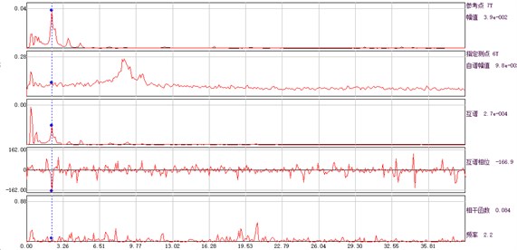
According to the displacement time history obtained from the ambient vibration test, the amplitude, phase and coherence function of the auto cross power spectrum of the response point and the reference point can be calculated, and the spectral line is illustrated in Fig. 4. The average periodogram method is used to calculate the power spectral density function, and the data point of fast Fourier transform is 1024. Hamming window is added, the window length is 1024, and the data overlap rate is 50 %.

Fig. 4Amplitude, phase and coherence function curve of auto and cross power spectrum of each measuring point and base point

a) Measuring point 1# and base point

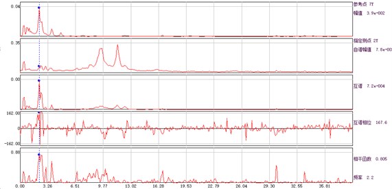
b) Measuring point 2# and base point

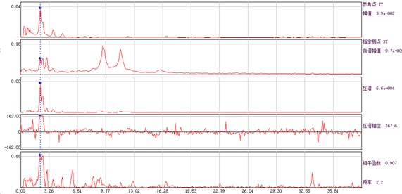
c) Measuring point 3# and base point

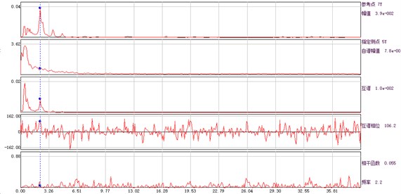
d) Measuring point 4# and base point

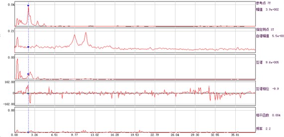
e) Measuring point 5# and base point

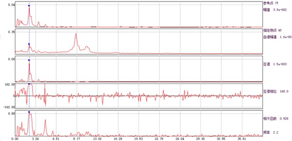
f) Measuring point 6# and base point

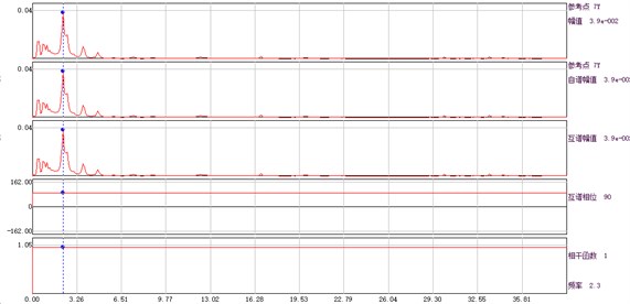
g) Measuring point 7# and base point

The identified first three frequencies and modes by using the auto and cross power spectrum method are shown in Table 1. For the convenience of finite element model updating, the standard vectors are normalized in this paper.

3.1. Arrangement of settlement monitoring points

The settlement of aqueduct is measured by static leveling method, and the monitoring points are arranged on the middle line of pedestrian passage on both sides of aqueduct. The monitoring point HX Base-1 is located at the mountain at the downstream end of aqueduct, and the other measuring points are located at the 1/4 span, 1/2 span, 3/4 span and two ends of each span. The arrangement of 46 monitoring points is showed in Fig. 5.

Fig. 5Arrangement of monitoring points for settlement observation

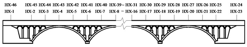
a) Vertical section

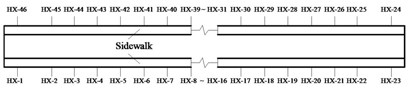
b) Plan section

3.2. Test methods and results

One vertical displacement reference point (HX Base-1) is set at both ends of the suspension span far away from the aqueduct, where the geological conditions are favorable and stable. HX base-1 and 45 monitoring points form a vertical displacement monitoring network. Observation is carried out according to first-class leveling requirements, and precision index is carried out according to second-class leveling standards. In the case the aqueduct stops flowing water and there exists no water, a closed line measurement can be made 12 hours later and recorded as the original data. After the aqueduct water flow reaches the stable value, it waits for 12 hours to measure and record the closed line, and the settlement data is obtained through data analysis based on the original record.

Before and after the aqueduct is flooded, the height difference of each measuring point relative to the base point (HQ Base-1) is measured respectively, and the settlement deformation data of aqueduct is obtained. Fig. 6 shows the vertical displacement of each measurement point.

Fig. 6Measured vertical displacements of the aqueduct

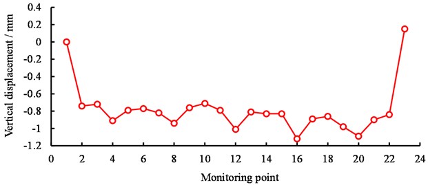
a) Monitoring point on the left sidewalk (HX1~HX23)

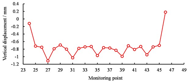
b) Monitoring point on the right sidewalk (HX24~HX46)

4.1. Objective function

Based on the measured vibration frequency and the measured vertical displacement, a multi-objective function is constructed. The objective function can be expressed as:

where, $f_{ai}$ and $f_{ti}$ are the calculated and measured $i$th order frequency of the aqueduct with empty resevior, respectively; $U_{aj}$ and $U_{tj}$ are the calculated and measured vertical displacement at the $j$th point of the aqueduct with full resevior; $n$ is the order of measured frequency; and $m$ is the number of settlement monitering point.

Since the calculated mode order of the finite element model does not necessarily coincide with the measured mode order, to ensure the mode matching between the calculated and the measured mode, the Modal Assurance Criterion (MAC) [19] is adopted to match the mode. The MAC can be expressed as follows:

where, ${\mathbf{\varphi }}_a$, ${\mathbf{\varphi }}_b$ are the calculated and measured mode vectors, respectively. MAC varies from 0 to 1, and the closer the MAC is to 1, the better the correlation is.

4.2. Model updating scheme

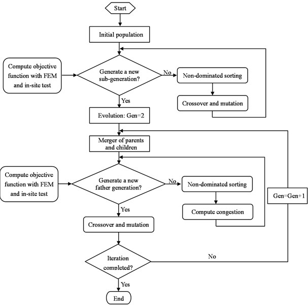
Based on the measured dynamic parameters of aqueduct and the settlement under the design water level, the non dominated sorting genetic algorithm [8] is used to optimize the multi-objective function and seek a non inferior solution. The specific implementation of model updating is to combine the optimization algorithm with the finite element analysis to realize the optimization solution. Fig. 7 shows the flow chart of the model updating scheme.

The population size of the multi-objective optimization algorithm is 60, the maximum number of evolution is 80, the crossover probability is 0.9, and the mutation probability is 0.1.

Fig. 7Flow chart of finite element model updating

5.1. Finite element model

Fig. 8 shows the finite element mesh of the aqueduct and its associated auxiliary components including top water channel and lower support arch bridge. The whole structures were discretized into 8-node hexahedron isoparametric elements. The finite element model contained 20698-node and 13905-element.

Fig. 8Finite element mesh

5.2. Model updating

5.2.2. Model updating results

Fig. 9 illustrates the relative correction of updated structural parameters. It can be seen that the rigidity and density of aqueduct body and the rigidity of the small arch ring change by more than 8%, while the other parameters change relatively little. Table 4 shows the static displacement and measured values of each span endpoint and mid-span point before and after the model updating. Measured settlement of each measurement point after the model updating is more consistent with the calculated settlement. The measured and calculated maximum displacements occurred in the middle of the fourth span (HX-16 measuring point). Before the model updating, the difference between the calculated and measured deflections is 17.0 %, and after the updating, the difference is reduced to 0.9 %; the maximum error between the calculated and measured deflections of the initial model occur at the top point of the fifth span bearing (HX-22 measuring point), which decrease from 81.8 % before the updating to 10.4 %. The dynamic characteristics and measured natural frequency before and after the model updating are shown in Table 5.

Fig. 9Relative correction of structural updating parameters / %

Table 4Comparison of settlement under design water level before and after model updating

Measuring points	Measured value/mm	Calculated value		Relative error/%
		Before updating	After updating	Before updating	After updating
HX-2	–0.73	–0.18	–0.71	75.3	2.7
HX-4	–1.01	–0.94	–1.02	6.9	1.0
HX-6	–0.73	–0.17	–0.69	76.7	5.5
HX-8	–0.99	–1.04	–1.05	5.1	6.1
HX-10	–0.73	–0.17	–0.70	76.7	4.1
HX-12	–0.99	–0.96	–1.00	3.0	1.0
HX-14	–0.80	–0.24	–0.75	70.0	6.3
HX-16	–1.06	–0.88	–1.05	17.0	0.9
HX-18	–0.84	–0.24	–0.80	71.4	4.8
HX-20	–1.02	–0.85	–1.04	16.7	2.0
HX-22	–0.77	–0.14	–0.69	81.8	10.4

Table 5Comparison of dynamic characteristics before and after model updating

Order	Frequency					MAC
	Measured / Hz	Calculated value / Hz		Relative error / %		Before updating	After updating
		Before updating	After updating	Before updating	After updating
1	2.25	2.25	2.25	0	0	0.75	0.83
2	2.54	2.43	2.54	4.3	0	0.72	0.83
3	2.93	2.83	2.92	3.4	0.3	0.72	0.82

It can be concluded that after the updating, the deviation between the calculated natural frequency and the measured value of each order is obviously reduced, and the degree of coincidence is higher. The MAC value of each order is also improved and the updated MAC is greater than 0.80. The first three modes of aqueduct after updating are shown in Fig. 10. In summary, the static and dynamic finite element model updating based on multi-objective optimization can achieve better results when applied to the masonry aqueduct structure.

Fig. 10First three modes of aqueduct

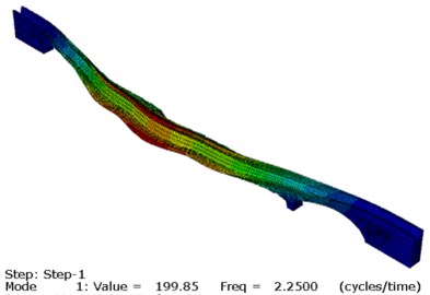
a) The 1st mode

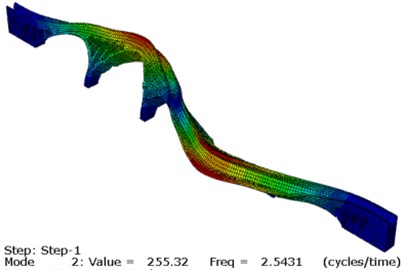
b) The 2nd mode

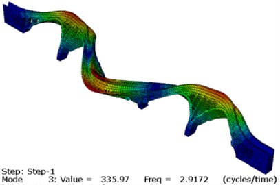
c) The 3rd mode