Abstract
Numerically simulated results by finite element model of a dynamic system do rarely coincide with the actual responses of the structure due to the modeling, manufacturing errors or other causes. The parameters of the finite element model should be corrected for subsequent proper analysis. Minimizing a cost function by the difference between the analytical and actual dynamic stiffness matrices along with constrained conditions of measured FRFs (Frequency Response Functions), this work provides the mathematical form on the updated FRF. The updated parameter matrices of the structure are derived from the FRF variation within the prescribed frequency range. It is shown that the exactness of the proposed method depends on the number of the measured data. The validity of the proposed method is illustrated in updating the parameter matrices of a planar truss structure.
1. Introduction
Finite element modeling should be established so that it can accurately predict the dynamic and static characteristics of real structural or mechanical systems under any disturbances. Any subsequent analysis based on the inaccurate finite element model may be flawed without any modeling correction because measured and analytical data are unlikely to be equal due to measurement noise, manufacturing errors and model inadequacies.
Structures can be modeled as discrete systems with the assumption of homogeneous and uniform systems without any defect, and the finite element analysis can be used to approximate the dynamic and static behavior of the systems. Before using a finite element model, it should be correlated with experimental data to ensure that it models the dynamics of the real structure. If that’s not the case, then it must be updated so that its dynamic responses more closely match the real structure dynamics. The update of physical parameter matrices of a finite element model concerns updating an analytical finite element model using measured data from a real life and experimental structure. However, it is impossible to experimentally obtain a full set data for a dynamic system. The data should be expanded to obtain the information on the whole system. The updated model must fulfill the constraints of the desirable physical and structural properties of the original finite element model.
Modal data or FRF data are utilized as measured data of the dynamic system. There have been many analytical methods for correcting analytical models to predict test results more closely [1-8]. Most of these methods have utilized the method of Lagrange multipliers utilizing the measured modal data. They are performed by minimizing a norm to use the weighting matrix in the satisfaction of constraints such as the orthogonality relationship and the eigenfunction of modal data.
FRF data provides more information than modal data, as the latter are extracted from a very limited frequency range related to resonance. Arora et al. [9, 10] considered the basic formulation for the complex parameter based updating method and its use for dynamic design. Based on the localization of modeling errors, Liu and Yuan [11] presented the methods to update the damping and stiffness matrices of damped systems with localized modeling errors. Imregun et al. [12] provided the basic formulation for the FRF based on the updating method and extended it to deal with complex FRF data. Lin and Zhu [13] developed an analytical method to identify damping matrices of structural systems, as well as mass and stiffness matrices. They established complex updating formulations using FRF data to identify damping coefficients for proportional damping and non-proportional damping. Arora et al. [14] worked on the update of finite element model using the FRF data with damping identification using complex modal data. By this method mass and stiffness matrices are firstly updated using a FRF-based model updating method and then damping is identified using updated mass and stiffness matrices. Inverting the FRF matrix to the dynamic stiffness matrix and comparing their real and imaginary parts with parameter matrices, Lee and Kim [15] identified damping characteristics of the system in matrix forms directly from its measured FRFs. Fritzen [16] proposed an analytical method to describe the parameter matrices by minimizing the error of dynamic stiffness matrix and its inverse, and identity matrix. Minas and Inman [17] identified the damping matrix based on the information of analytical finite element model and measured complex modal parameters. Nozarian and Esfandiari [18] presented a model updating method using FRF data and measured natural frequencies of the damaged structure without any expansion or reduction. Pascual et al. [19] presented a model updating method to avoid the numerical difficulties induced by the discontinuities in the FRFs. Esfandiari et al. [20, 21] provided a structural model updating technique using measured FRF data and measured natural frequencies of the damaged structure without any expansion of the measured data or reduction of the finite element model. Using damage sensitivity equations by the least square method, they estimated the mass, stiffness and damping properties. Utilizing FRF data measured at specific positions, with dofs less than that of the system, as constraints to describe a damaged system, Rahmatalla et al. [22] identified parameter matrices such as mass, stiffness and damping matrices of the system, and provided a damage identification method from their variations.
This work begins with FRF data measured at a few positions rather than modal data. Minimizing a cost function by the difference between the actual and analytical dynamic stiffness matrices, and using the constrained conditions of measured FRF data, this study provides a mathematical form to predict the FRF matrix of a full set of dofs. The parameter matrices of the dynamic system are updated from the predicted FRF matrix within the prescribed frequency range. It is shown that the exactness of the proposed method depends on the number of the measured data. The update of the parameter matrices of a planar truss structure is considered for proving the validity of the proposed method.
2. Formulation
Using the finite element method, the dynamic equation of forced motion for a damped dynamic system is expressed as a system of a second-order differential equation. The dynamic response of a structure which is assumed to be linear and approximately discretized can be described by the equations of motion:
where , and denote the analytical mass, damping, and stiffness matrices, , and is the external force vector.
Assume the displacement vector and the external force vector of Eqn. (1) in exponential forms of:
where denotes the modal coordinate vector, is an excitation force vector, is the excitation frequency and . The substitution of Eq. (2) into Eq. (1) yields the equation:
The equilibrium equation of the analytical model can be expressed as:
where . The displacement vector is calculated by:
In order to update the FRF and parameter matrices of the structure, measured data should be utilized as the basic information for the correction because it is impractical to measure the displacements at all positions. Assume that the displacements measured at positions corresponding to different force sets at a frequency were measured. The measured displacements are written as:
where is an Boolean matrix to define the measurement positions. denotes an displacement matrix of the actual structure and represents an measured data of where is the measured FRF matrix. where denotes the -th unitary vector of excitation with an element being unit and all other elements zeros.
Substituting into Eqn. (6), it follows that:
where is an dynamic stiffness matrix to be updated. This work derives the dynamic stiffness matrix by minimizing a cost function of the difference between the analytical stiffness matrix and the actual stiffness matrix .
The updated dynamic stiffness matrix is estimated by a least square method utilizing a cost function of:
In order to utilize Eqn. (7) into Eqn. (8), Eqn. (7) is modified as:
Letting and , and solving the result with respect to , we obtain that:
where the superscript ‘+’ indicates the Moore-Penrose inverse and is an arbitrary matrix. We can recognize that there are an infinite number of solutions on the actual stiffness matrix due to the presence of the arbitrary matrix . We derive the FRF matrix to satisfy the condition to minimize the cost function of Eq. (8) of all solutions of Eq. (10). Utilizing the condition to minimize Eq. (8) into Eq. (10) and solving it with respect to the arbitrary matrix, it is derived as:
where is an arbitrary matrix. Utilizing Eq. (11) into Eq. (10), the following equation is obtained as:
Again, solving Eq. (12) with respect to , it is derived as:
where is an arbitrary matrix.
Inserting the condition to minimize Eq. (8) into Eq. (13) and solving the result with respect to the arbitrary matrix, we obtain:
where is an arbitrary matrix. The substitution of Eq. (14) into Eq. (13) yields:
Premultiplying and postmultiplying both sides of Eq. (15) by , the updated flexibility matrix of the damaged system can be expressed as:
The inverse of the flexibility matrix of Eq. (16) represents the updated dynamic stiffness matrix derived from the assumption utilized in this study. Expressing Eq. (16) in the terms of the flexibility matrices, and , it can be written as:
where and represent the flexibility matrices of updated system and finite element model, respectively. indicates the variation in the FRF matrix between two systems. The physical parameters can be grasped by investigating the variation in FRF matrix.
The parameter matrices are calculated from the estimated FRF matrix of Eq. (17):
Taking the first-order approximation on the last equation in Eqn. (18) and using the relation of , it is expressed by:
Substituting the FRF matrix defined in Eqn. (3) into Eqn. (19), the variation in FRF matrix is derived:
The FRF matrix is composed of real and imaginary parts. Partitioning the equation of the left-hand side in Eqn. (20) in terms of real and imaginary parts, they can be written as:
where and indicate the real and imaginary parts, respectively. It is shown that the stiffness and mass matrices of dynamic system are strongly related to each other.
Assuming that distinct frequency responses corresponding to excitation frequencies denoted by are experimentally measured, the relations of Eq. (21) are expanded as:
where:
Solving Eq. (22) with respect to the parameter matrices, they follow:
The corrected parameter matrices can be obtained by:
Eq. (24) denote the parameter matrices estimated from this method in the satisfaction of the incomplete FRF data. The FRF data at the unmeasured dofs were estimated from the measured FRF data and dynamic equations of the finite element model. If we collect all information at the full set of dofs, the predicted FRF will coincide with the actual one. However, the prediction of the FRF matrix based on a few measured data can lead to inconsistency with the actual one. It will be evaluated that the predicted FRF matrix and parameter matrices proposed in this study properly describe the actual ones through numerical experiments.
3. Application
The inconsistency between the actual and analyzed responses requires the correction of the parameters of the modeled structure. Using the proposed method, this application handles the correction of the parameter matrices of a plane truss structure model shown in Figure 1. In the figure, the nodal points and the members are numbered as shown in the figure. The truss is composed of 15 nodes and 33 members. All members have elastic modulus of 200 GPa, cross-sectional area of 2.5×10⁻³ m2, and density of 7860 kg/m3. For this numerical experiment, we assumed that the mass and stiffness of the actual members include some errors shown in Tables 1 and 2, respectively. The errors of stiffness and mass of each member were randomly selected in the range of 0-20 % loss.
Fig. 1A planar truss structure
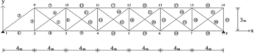
Table 1Reduction percentage of the mass of all members (%)
6.3 | 4.1 | 4.6 | 4.1 | 4.9 | 7.8 | 5.7 | 2.8 | 1.1 | 0.2 | 0.4 |
4.5 | 0.6 | 4.7 | 0.7 | 0.5 | 6.2 | 6.1 | 0.1 | 7.2 | 0.4 | 1.7 |
8.0 | 1.2 | 2.1 | 6.1 | 0.4 | 9.9 | 4.8 | 16.0 | 2.1 | 1.7 | 4.4 |
Table 2Reduction percentage of the stiffness of all members (%)
6.4 | 2.7 | 1.8 | 4.7 | 7.4 | 1.4 | 5.6 | 4.7 | 8.2 | 1.5 | 6.0 |
1.4 | 2.5 | 3.9 | 2.3 | 3.5 | 0.5 | 3.8 | 17.7 | 7.3 | 1.2 | 13.4 |
0.6 | 10.4 | 0.03 | 7.4 | 3.0 | 1.5 | 1.0 | 0.4 | 6.3 | 3.5 | 3.9 |
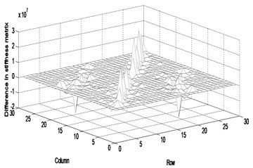
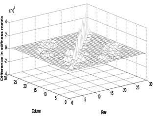
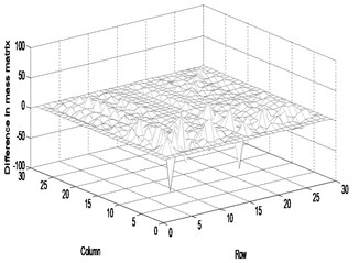
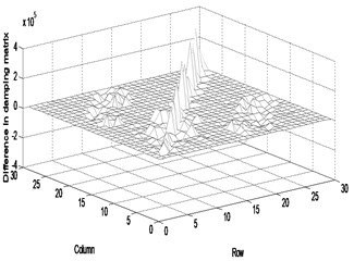
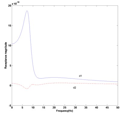
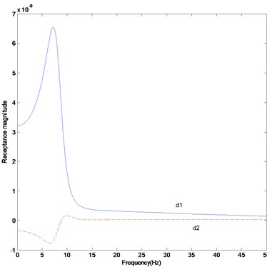
Fig. 2Difference in the parameter matrices between the actual and updated systems (fifteen measurement data): a) stiffness, b) mass, c) damping
a)
b)
c)
Table 3The first five natural frequencies (rad/sec)
1st | 2nd | 3rd | 4th | 5th | |
Finite element model | 55 | 162 | 225 | 413 | 569 |
Actual system | 54 | 160 | 223 | 413 | 562 |
Updated system | 53 | 160 | 225 | 414 | 568 |
Table 4The first five natural frequencies (rad/sec)
1st | 2nd | 3rd | 4th | 5th | |
Finite element model | 55 | 161.8 | 224.5 | 412.6 | 569.2 |
Actual system | 54.9 | 162.2 | 223.8 | 412.3 | 569.3 |
Updated system | 54.9 | 162.1 | 223.3 | 414.1 | 569.3 |
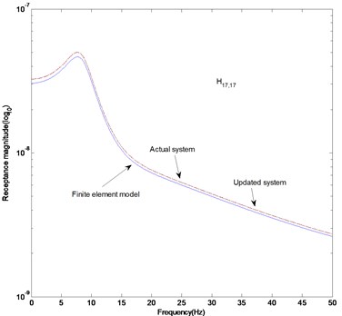
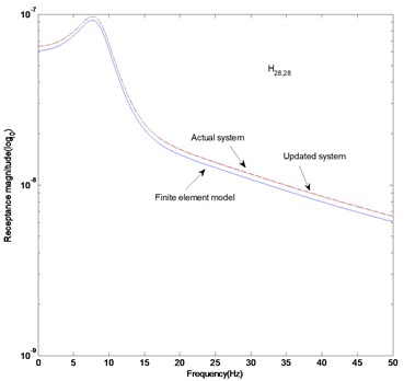
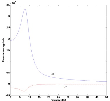
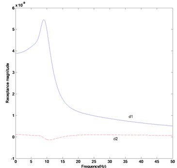
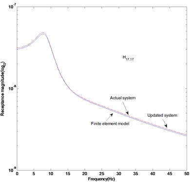
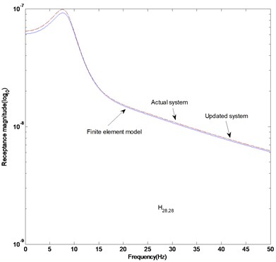
Fig. 3FRF curves (fifteen measurement data): a) H17,17, b) H28,28, c) difference in receptance magnitude H17,17, d) difference in receptance magnitude H28,28
a)
b)
c)
d)
The modal displacements at fifteen positions of total twenty-seven dofs besides the boundary conditions were selected as the measurement data corresponding to ten excitation sets. The fifteen measurements include , , , , , , , , , , , , , and , where and represent the horizontal and vertical displacements, and the subscript denotes the node number. Firstly, the FRF variation between the actual system and the finite element model was estimated using Eqn. (17) and the noise-free measurement data in the range of 8.4-8.8 Hz in steps of 0.02 Hz. The parameter matrices were corrected from the calculated FRF matrix using Eqns. (23). Table 3 compares the first five natural frequencies of finite element model, actual system and updated system by the proposed method. The table shows a very little difference in the natural frequency between the finite element model and actual system, and the actual and updated systems. However, the difference between the actual and updated systems increases very little with the number of modes. It is expected that the difference comes from the estimation of the FRF and parameter matrices at the unmeasured positions. Figure 2 exhibits the difference in the parameter matrices of stiffness, mass and damping between the actual and updated systems. The FRF response data are obtained by the roving of accelerometer under the excitation of the impact hammer at reference points corresponding to , , , , , , , , and . The mathematical solution of the parameter matrices estimated in this method is the one to minimize the cost function of the infinite number of solutions to satisfy the measurement data as recognized from the arbitrary matrix in Eqn. (10). The parameter matrices of the actual truss system and the updated system can be the ones of all the solutions to satisfy the measurement data. It is explained that the inconsistency comes from less number of measurement data than the number of dofs. If the measurement data at a full set of dofs are given, the parameter matrices will be uniquely predicted.
Fig. 4Difference in the parameter matrices between the actual and updated systems (twenty measurement data): a) stiffness, b) mass, c) damping
a)
b)
c)
The parameter matrices established in this study are the solutions to satisfy the measurement data of the dynamic system. They explain the dynamic characteristics of the whole system rather than the local characteristics such as stiffness, mass and other dynamic properties. The results can be proved from Figs. 3 (a) and (b) to depict the FRF magnitude at the 17th row and 17th column, and 28th row and 28th column in the FRF matrix. It is observed that the FRF magnitudes of the actual and updated systems are almost the same. Figures 3 (c) and (d) display that the receptance magnitude between the actual system and finite element model, , results in slightly larger difference than the one between the actual and updated systems, . We have to consider the increase in the measurement data to enhance the exactness of the estimated parameter matrices.
Fig. 5FRF curves (twenty measurement data): a) H17,17, b) H28,28, c) difference in receptance magnitude H17,17, d) difference in receptance magnitude H28,28
a)
b)
c)
d)
As in the second case, we considered the update of the parameter matrices using more measurement data than the previous case. The twenty measurements include , , , , , , , , , , , , , , , , , , and . The FRF response data are obtained by the roving of accelerometer under the excitation of the impact hammer at reference points corresponding to , , , , , , , , and . We also assumed the errors not to be the same errors as the previous case. Tables 3 and 4 exhibit that the natural frequencies of the updated system are closer to the ones of the actual system when the number of the measurement data increases from fifteen to twenty. It is explicitly found from the comparison of Figs. 2 and 4 that the difference in the parameter matrices between the actual and updated systems decreases very slightly with the increase in the number of measurement data. However, the inconsistency exists and the parameter matrices proposed in this study should be the ones of all parameter matrices to satisfy the measurement data. If the number of the measurement data is less than the number of dofs, the inconsistency will exist. Figures 5(a) and (b) show that the actual FRF curve almost coincides with the estimated FRF curve. The receptance magnitude between the actual system and finite element model, , yields slightly larger difference than the one between the actual and updated systems, as shown in Figs. 5(c) and (d). It is shown from the comparison of Figs. 3(c) and (d) and 5(c) and (d) that the gap between two curves reduces with the increase in the number of the measurement data. As the result, the proposed method properly explains the global characteristics of the system, but leads to some inconsistency between the actual and estimated parameter matrices. The inconsistency will be overcome by increasing the number of measurement data.
4. Conclusions
This work provided the mathematical form on the variation of FRF matrix by minimizing a cost function of the difference in the dynamic stiffness matrix between the actual system and the finite element model. The measurement data were utilized as the constraints for deriving the estimated FRF matrix. The parameter matrices were predicted from the estimated FRF matrix. The inconsistency of the parameter matrices between the actual and updated systems comes from a less number of measurement data than the number of dofs. Because the updated parameter matrices can be ones of the solutions to utilize the measurement data as the constraint condition, they rarely affect the dynamic characteristics of the global system but the updated parameter matrices. If the measurement data at a full set dofs are given, the parameter matrices will be uniquely predicted. The increase in the measurement data will enhance the exactness of the estimated parameter matrices.
References
-
Kabe A. M. Stiffness matrix adjustment using mode data. AIAA Journal, Vol. 23, 1985, p. 1431-1436.
-
Lee U., Shin J. A frequency response function-based structural damage identification method. Computers & Structures, Vol. 80, 2002, p. 117-132.
-
Baruch M., Bar-Itzhack I. Y. Optimal weighted orthogonalization of measured modes. AIAA Journal, Vol. 16, 1978, p. 346-351.
-
Baruch M. Optimal correction of mass and stiffness matrices using measured modes. AIAA Journal, Vol. 20, 1982, p. 1623-1626.
-
Berman A. Mass matrix correction using an incomplete set of measured modes. AIAA Journal, Vol. 17, 1979, p. 1147-1148.
-
Caeser B., Pete J. Direct update of dynamic mathematical models from modal test data. AIAA Journal, Vol. 25, 1987, p. 1494-1499.
-
Berman A., Nagy E. J. Improvement of a large analytical model using test data. AIAA Journal, Vol. 21, 1983, p. 1168-1173.
-
Friswell M. I., Mottershead J. E. Finite Element Model Updating in Structural Dynamics. Kluwer Academic Publishers, 1995.
-
Arora V., Singh S. P., Kundra T. K. On the use of damped updated FE model for dynamic design. Mechanical Systems and Signal Processing, Vol. 23, 2009, p. 580-587.
-
Arora V., Singh S. P., Kundra T. K. Damped model updating using complex updating parameters. Journal of Sound and Vibration, Vol. 20, 2009, p. 438-451.
-
Liu H., Yuan Y. New model updating method for damped structural systems. Computers and Mathematics with Applications, Vol. 57, 2009, p. 685-690.
-
Imregun M., Visser W. J., Ewins D. J. Finite element model updating using frequency response function data – I: Theory and initial investigation. Mechanical Systems and Signal Processing, Vol. 9, 1995, p. 187-202.
-
Lin R. M., Zhu J. Model updating of damped structures using FRF data. Mechanical Systems and Signal Processing, Vol. 20, 2006, p. 2200-2218.
-
Arora V., Singh S. P., Kundra T. K. Damped FE model updating using complex updating parameters: its use for dynamic design. Journal of Sound and Vibration, Vol. 324, 2009, p. 1111-1123.
-
Lee J. H., Kim J. Identification of damping matrices from measured frequency response functions. Journal of Sound and Vibration, Vol. 240, 2001, p. 545-565.
-
Fritzen C. P. Identification of mass and stiffness matrices of mechanical systems. Journal of Vibration and Acoustics, Vol. 108, 1986, p. 9-16.
-
Minas C., Inman D. J. Identification of a nonproportional damping matrix from incomplete modal information. Journal of Vibration and Acoustics, Vol. 113, 1991, p. 219-224.
-
Nozarian M. M., Esfandiari A. Structural damage identification using frequency response function. Materials Forum, Vol. 33, 2009, p. 443-449.
-
Pascual R., Schalchli R., Razeto M. Damping identification using a robust FRF-based model updating technique. XXI International Modal Analysis Conference, 2003.
-
Esfandiari A., Bakhtiari-Nejad F., Rahai A., Sanayei M. Structural model updating using frequency response function and quasi-linear sensitivity equation. Journal of Sound and Vibration, Vol. 326, 2009, p. 557-573.
-
Esfandiari A., Bakhtiari-Nejad F., Sanayei M., Rahai A. Structural finite element model updating using transfer function data. Computers & Structures, Vol. 88, 2010, p. 54-64.
-
Rahmatalla S., Eun H. C., Lee E. T. Damage detection from the variation of parameter matrices estimated by incomplete FRF data. Smart Structures and Systems, Vol. 9, 2012, p. 55-70.
About this article

This research was supported by the Chung-Ang University Research Scholarship Grants in 2012.
