Investigation of the stability of fluctuations in electrocardiography data

1. Introduction

During the last years studies of the complexity in human body functioning prove to be an important area of research [1]. An integral evaluation model [2] based on the combination of the main functional holistic [3] systems of the human body – skeletal and muscle system (the performing system), cardiovascular system (the supplying system) and central nervous system (the regulatory system) has been developed several decades ago. Thus, all the three systems always react together during the adaptation processes in a human body; the general reaction of the body is always the combination of these systems’ responses. Reactions of the cardiovascular system to a constant load test (or a gradually increasing load test) can reveal the peculiarities of the functioning of all human body [4]. ECG parameters have different duration (larger structures could be associated with longer time scales) and could show the complexity in different fractal levels [5].

A number of techniques have been used for the analysis of ECG complexity: spectral analysis [6], entropy-based algorithms (as for example, approximate entropy [7, 8], sample entropy [9, 10], multiscale entropy [1]), chaos-based algorithms (as for example, Lyapunov exponent [11], permutation entropy [12], Hankel matrix [10]), algorithms for Komologrov estimates (as for example, Lempel-Ziv [13], hidden Markov chains [14]) and other methods. These methods evaluate global features of processes and are not able to detect local features of dynamical processes.

The rank of a sequence has been exploited for the evaluation of the complexity of certain ECG parameters [10]. Also, it has been used to express solutions of nonlinear differential equations in forms comprising ratios of finite sums of standard functions [15-17] and for the identification of the skeleton algebraic progression in time series [18, 19].

The main objective of this paper is to propose an algebraic algorithm based on the concept of the rank of a sequence [20] for the analysis of ECG signals. Our goal is to develop a strategy for finding the nearest algebraic progression to each segment of time series of the ECG parameters. We will suppose that the proposed algebraic algorithm can be effectively used for the analysis of ECG parameters.

The developed algebraic algorithm was applied for the analysis of physiological processes in a bicycle ergometry test. ECG parameters of different durations were used for the investigation of dynamics of different physiological processes in human heart during the load.

2. The concept of the rank of a sequence

Let us consider a sequence: $p_0,p_1,p_2,...:=(p_j;j\in Z_0)$ where elements $p_j$ can be real or complex numbers. Then the sequence of Hankel matrixes is read as:

The Hankel transform (the sequence of determinants of Hankel matrixes) $(d_n;n\in N)$ reads:

Definition 1. The sequence $(p_j;j\in Z_0)$ has a rank $m\in Z_0$; $m<+\infty$:

if the sequence of determinants of Hankel matrixes has the following structure:

where $d_m\ne 0$ and $d_{m+1}=d_{m+2}=...=0$.

Example 1. Let’s say $p_j:=j^2$; $j\in Z_0$. Then, $Hr(j^2;j\in Z_0)=3$ because the sequence of determinants of Hankel matrices reads $(0,-1,-\mathrm{8,0},0,\dots )$.

Definition 2. Let $Hr(p_j;j\in Z_0)=m$. Then the characteristic Hankel determinant for the sequence $(p_j;j\in Z_0)$ is defined as [10]:

The expansion of the determinant in Eq. (5) yields an $m$th order algebraic equation for the determination of roots of the characteristic equation:

where $A_m\ne 0$ because $A_m=d_m\ne 0$.

We have assumed, that ${\mu }_{rg}\left(\begin{array}{c}j\\ g\end{array}\right){\rho }_r^{j-g}=0$ if $\left(\begin{array}{c}j\\ g\end{array}\right)=0$ what is true when $0\le j<g$. Moreover, $0^0=1$; $0^1=0^2=...=0$. Then the following theorem holds.

Theorem 1. Let $Hr(p_j;j\in Z_0)=m$ and the recurrence indexes of roots ${\rho }_1,{\rho }_2,{\rho }_3,...,{\rho }_c$ of the characteristic equation (Eq. (6)) are $m_1,m_2,...,m_c(c=\mathrm{1,2},3,...)$ accordingly; $\sum _{r=1}^c{m}_r=m$. Then the following equality holds true:

The opposite statement also holds. If Eq. (7) holds true, then:

$Hr(p_j;j\in Z_0)=m_1+m_2+...+m_c.$

Rigorous proof of this theorem is given in [10].

Definition 3. A sequence $(p_j;j\in Z_0)$ is an algebraic progression if elements of that sequence can be expressed in the form of Eq. (7).

Corollary 1. Eq. (7) can be rewritten in the following form:

where ${\rho }_1,{\rho }_2,...,{\rho }_c\ne 0$; ${\mu }_{r{m}_r-1}\ne 0$ and ${\widehat{\mu }}_{rg}$ do not depend on $j$.

Corollary 2. In case when all roots of the characteristic equation are different, Eq. (7) obtains a more simple form:

It can be also noted that coefficients ${\mu }_{rg}$ (or just ${\mu }_r$) can be found solving the linear algebraic system of equations (${\rho }_1,{\rho }_2,...,{\rho }_c$ are determined beforehand):

This linear system of algebraic equations has one and the only one solution [20].

Corollary 3. Let $Hr(p_j;j\in Z_0)=m$ and the first $2m$ elements of that series are known. Then it is possible to use Eq. (6), Eq. (10) and Eq. (7) to calculate all elements of that sequence.

Corollary 4. Suppose Eq. (3) holds true. It can be stated that accordingly to Eq. (8) the following equality holds true:

where ${\rho }_1,{\rho }_2,...,{\rho }_c\ne 0$; ${\mu }_{r{m}_r-1}\ne 0$; ${\tilde{\mu }}_{rg}{\rho }_r^k$ do not depend on $j$ and:

Consequently, the rank of the subsequence $(q_j;j\in Z_0)$ with all $k\in Z_0$, $h\in N$ is equal to:

Next, the inverse task will be needed. It is important to obtain the algebraic progression of sequence $p_j,j\in Z_0$ then an algebraic progression $q_j$ (Eq. (11)) and parameters $h$, $k$ are determined. Thereby, accordingly to Eq. (12) ${\rho }_r$ can be expressed in the form:

where $\left|{\tilde{\rho }}_r\right|\ge 0$, $\sqrt[h]{\left|{\tilde{\rho }}_r\right|}\ge 0$ and $-\pi \le \mathrm{a}\mathrm{r}\mathrm{g}{\tilde{\rho }}_r<\pi ,a=\mathrm{0,1},...,h-1.$

But value of ${\rho }_r$ it is the only possible (it is then $a=a_0$) in the algebraic progression of $p_j,j\in Z_0$:

where values ${\left({\rho }_r\right)}_{a_0}$ can be selected minimizing the root mean square error (RMSE):

where $\eta \in N$ which allows to estimate the value of $a_0$.

It should be noted that coefficients ${\widehat{\mu }}_{rg}$ (Eq. (15)) can be found by solving the linear algebraic system of equations.

Corollary 5. It can be admitted that the concept of the rank of the sequence given above can be applied to finite length sequences in practice. If the sequence $(p_0,p_1,...,p_{L-1})$ of length $Li$ is given so the sequence of Hankel matrices is: $H_1,H_2,...,H_n,n\le L/2$. We have to assume that the rank of the sequence is not defined if $d_n\ne 0,n\le L/2$.

Corollary 6. In application of Theorem 1 it is important to distinguish the:

a) ${\omega }_j^{\left(0\right)}=\sum _{k:\left|{\rho }_k\right|=1}{\mu }_k{\rho }_k^j,j\in Z_0$ - stationary component;

b) ${\omega }_j^{\left(1\right)}=\sum _{k:\left|{\rho }_k\right|>1}{\mu }_k{\rho }_k^j,j\in Z_0$ - stimulant component;

c) ${\omega }_j^{(-1)}=\sum _{k:\left|{\rho }_k\right|<1}{\mu }_k{\rho }_k^j,j\in Z_0$ - inhibitory component;

of time series which consists of the complexity of content of time series:

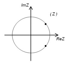
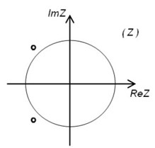
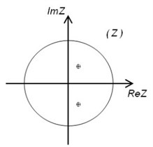
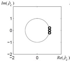
It must also be stated that roots ${\rho }_1,{\rho }_2,{\rho }_3,...,{\rho }_c$ of the characteristic equation (Eq. (6)) can be placed on the unit circle (Fig. 1).

Fig. 1a) – stationary behavior – on the unit circle |z|= 1; b) – stimulant behavior – outside of the unit circle |z|=1, c) – inhibitory roots are inside the unit circle |z|= 1

a)

b)

c)

Example 1. Let us consider the following sequences:

a) $x_j=10\mathrm{c}\mathrm{o}\mathrm{s}\left(0.1j\right)+40\mathrm{s}\mathrm{i}\mathrm{n}\left(0.2j\right),j\in Z_0$,

b) $y_j=2\mathrm{c}\mathrm{o}\mathrm{s}\left(0.2j\right)e^{0.5j}+e^{0.3j},j\in Z_0$,

c) $w_j=200\mathrm{s}\mathrm{i}\mathrm{n}\left(0.3j\right)e^{-0.2j}+45\mathrm{c}\mathrm{o}\mathrm{s}\left(0.1j\right)e^{-0.5j},j\in Z_0$.

Let us compute the rank and find roots ${\rho }_1,{\rho }_2,{\rho }_3,...,{\rho }_c$ of the characteristic equation (Eq. (6)) of sequence $x_j$,$j\in Z_0$. It is clear that $Hr(x_j;j\in Z_0)=4$ because the sequence of determinants of Hankel matrices reads: $(\text{1, 10}\text{, -}\text{66.52, -0.57},\mathrm{0,0},\dots )$. Then Hankel algebraic equation (Eq. (6)) is:

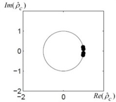
Its roots are: ${\widehat{\rho }}_{\mathrm{1,2}}=0.9801\pm 0.1987i$, ${\widehat{\rho }}_{\mathrm{3,4}}=0.9950\pm 0.0998i.$ Roots are placed on the unit circle (Fig. 2, (a)).

Analogously, roots $({\rho }_1,{\rho }_2,{\rho }_3,...,{\rho }_c)$ can be found from the characteristic equations for other sequences $y_j$, $w_j$, $j\in Z_0$.

Note that the given sequence $x_j$ has a stationary component because its roots are located on the unit circle (Fig. 2(a)), the sequence $y_j$ – a stimulant component because its roots are placed outside the unit circle (Fig. 2(b)), and the sequence $w_j$ – an inhibitory component as its roots are placed inside the unit circle (Fig. 2(c)).

Fig. 2The location of the roots of the Hankel algebraic equation for each given sequence a), b) and c)

a)

b)

c)

3. Algebraic method for the analysis of ECG parameter

Let us assume that $P=(p_0,p_1,...,p_{L-1})$ is the time series of ECG parameters of length $L$ consisting of several segments of algebraic progressions (Eq. (7)). We will construct algebraic method for the ECG parameter analysis.

The segmentation algorithm for algebraic progressions is constructed in [9] where numerical sequences (without noise) were segmented into non-overlapping contiguous segments by constructing algebraic progressions of each segment. Unfortunately, time series of ECG parameters usually are noisy and the proposed method can’t be applied directly.

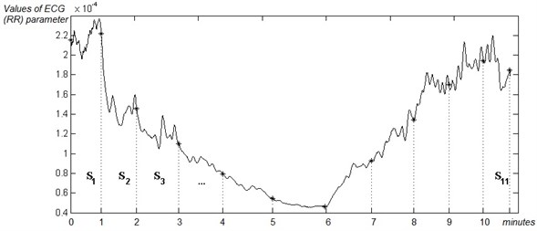
Let a time series of ECG parameters $P$ be segmented manually into $k$ non-overlapping contiguous segments $S_l=S_l(u_l,v_l)=(p_{u_l},p_{u_l+1},....,p_{v_l})$, $u_l\le v_l(S:=\underset{l}{\cup }{S}_l,l=\stackrel{-}{1,k})$ where $u_l$ is the start and $v_l$ – the end position of each segment $S_l$ (Fig. 3). Let us construct an algorithm for finding algebraic progression of each segment $S_l$.

Let us assume that $m_t$ is the rank (then Theorem 1 can be applied), $k_t$ is the start position and $h_t$ – the step of the regular grid in the interval of the subsequence $P_t\subset P.$ Then we can construct $t$ different subsequences $P_t=p_{k_t+h_{t}j}$,$j=\stackrel{-}{0,b_t-1}$, $b_t=2m_t{h}_t$, with different combinations of parameters $m_t$, $k_t$ and $h_t$ can be generated according to equality: $g_t=k_t+2m_t{h}_t-h_t$, where $g_t$ – is the given last position of subsequence $P_t$.

It can be noted that correspondingly to Eq. (11) $t$ different algebraic progressions of each subsequence $P_t$ can be observed:

Fig. 3The segmentation of an ECG signal into k non-overlapping contiguous segments

Let us construct an algebraic progression Eq. (18) of subsequence $P_t$. We have assumed that the rank of the algebraic progression $q_j^{\left(t\right)}$ is $m_t$ and parameters $k_t$, $h_t$ are known (the initial step of the regular grid in the interval of each subsequence must be at least $h_0=2$). Then the characteristic Hankel determinant (Eq. (5)) takes the form:

and yields roots ${\tilde{\rho }}_1^{\left(t\right)},{\tilde{\rho }}_2^{\left(t\right)},\dots ,{\tilde{\rho }}_{m_t}^{\left(t\right)}$. The linear system of equations is constructed using Eq. (8); its solution produces coefficients ${\tilde{\mu }}_r^{\left(t\right)}$; $r=\mathrm{1,2},\dots ,m_t$. Finally, the algebraic progression $q_j^{\left(t\right)}$ reads:

It can be concluded that according to Eq. (20), Eq. (12) and Eq. (15) algebraic progression of subsequence $P_t$ can be obtained:

We have assumed that Eq. (21) is the closest algebraic progression of segment $S_l$ if the following equality holds true:

where $R({\widehat{P}}_l,u_l^0,v_l^0)$ is the minimal value of $RMSE$ values; ${\widehat{P}}_l={\widehat{p}}_{k_l+h_{l}j}$, $j=\stackrel{-}{0,v_l^0-u_l^0-1}$, $u_l^{\text{0}}=k_l$ – the start and $v_l^0=u_l^0+2m_l{h}_l-h_l$ – the end positions of sequence ${\widehat{P}}_l$ and estimations: ${\widehat{m}}_l={\widehat{m}}_t$, ${\widehat{h}}_l={\widehat{h}}_t$, ${\widehat{k}}_l={\widehat{k}}_t$, where ${\widehat{m}}_t$, ${\widehat{k}}_t$, ${\widehat{h}}_t$ – estimations which were used to obtain the minimized algebraic progression ${\widehat{p}}_j^{\left(t\right)}$, $j\in Z_0$.

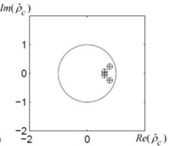
After all algebraic progressions of each given ECG fragment $S_l$ are known, depending on the parameter $\epsilon \ge 0$ (Fig. 4(a)) where the counts of roots placed outside are calculated, inside and on the unit circle of each segment $S_l$.

Fig. 4a) The location of roots of the algebraic progression for the segment S1, b) separation of components (roots) of algebraic progression of segment S1 depending on parameter ε= 0.01

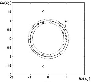
a)

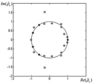
b)

Example 2. Providing the time series of RR parameter of ECG signal are given and the signal is manually segmented into 11 non-overlapping contiguous segments $S:=\underset{l}{\cup }{S}_l$, $l=1,..,11$ (Fig. 3) and all algebraic progression of each segment $S_l$, $l=1,..,11$ are found. Parameters of the algebraic progression of segment $S_1=S_1\left(\mathrm{1,96}\right)$ are presented in Table 1. Roots $({\widehat{\rho }}_1,{\widehat{\rho }}_2,{\widehat{\rho }}_3,...,{\widehat{\rho }}_{24})$ are placed on the unit circle (Fig. 4). It was calculated (with $\epsilon =0.01$) 5 stationary, 9 stimulant and 10 inhibitory components of the analyzed segment $S_1$ (Fig. 4(b)).

4. Experiment and results

Ten healthy participants (20,1 ± 2,23) volunteered to take part in this study, where a bicycle ergometry test was performed and the ECG was recorded continuously during the whole test of 12 leads synchronously. Only males with experience in sprint (practicing more than 2 years) were chosen, as the cardiovascular systems reactions to physical load differ with gender. This was done in order to obtain relatively homogenous group for getting more comparable data. When arriving at the laboratory, participants were asked to dress in shorts and wear trainers.

Before performing the bicycle ergometry test all the participants were informed verbally and all their questions were answered. All participants underwent the same test protocol which consisted of three main parts – rest, load and recovery. In this study the rest part took 1 minute while a participant was just sitting on the bike without pedaling. After the rest proceeded physical work that included computer-based bicycle ergometry test based on provocative incremental increase of the load. Bicycle ergometry test started with 50 W and in every minute the load was increased by 50 W. The test was continued up to 250 W that made 5 minutes of pedaling at 60 cycles per minute. Although the maximum load hasn’t been reached, the test should have been ended earlier if the distressing cardiovascular symptoms appeared. Finally, the last part of the protocol was recovery that took five minutes. The total time of the protocol lasted eleven minutes (Fig. 5-7). During the bicycle ergometry test electrocardiogram (ECG) was registered. For synchronous recording of 12-lead ECG a computerized ECG analysis system “Kaunas-load” was employed.

During rest, load and recovery were evaluated ECG parameters: RR interval (the interval between two beats of heart), JT interval (interval corresponds to the electric systole of heart and the shortening of JT interval is associated with intensity of metabolic processes in heart), QRS complex (describes inner heart regulation system).

The aim of this experiment was to explore the local changes of different ECG parameters in dynamic.

It is necessary to remind that ECG parameters that are examined reveal different complexity levels, e.g. RR interval helps to characterize the state of organism in regulatory level, JT interval represents the metabolic reactions of the systems and QRS reflect the intrinsic regulatory state of the organ.

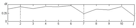
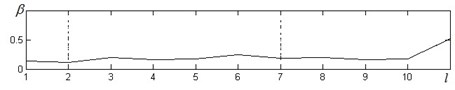
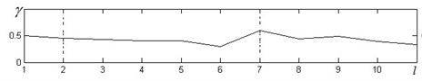
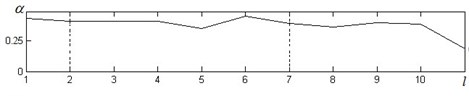
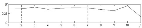
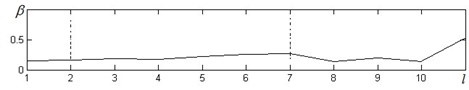
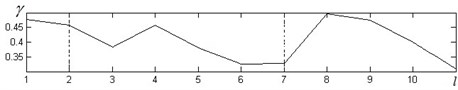
The test was performed in eleven minutes where 1 minute represented rest interval, 2-6 the load minutes and 6-11 were the interval of recovery of the test (figure 5-7 x-axes). In every minute of the test the normalized values of those different processes (inhibitory (value -$\alpha$), stationary (value -$\beta$) and stimulant (value -$\gamma$)) were calculated (y-axes) dividing Hankel algebraic equation roots of each process by the total number of Hankel algebraic equation roots which were placed on the circles. The procedure to find normalized values of inhibitory, stationary and stimulant process was separately performed for RR interval (Fig. 5), JT interval (Fig. 6) and QRS interval (Fig. 7).

From the data it can be seen that at the beginning of the physical load starts the inhibitory process begin to lead and is mostly expressed at the last minute of the load in this case it is an interval from minute 5 to 6, Fig. 5(a), Fig. 6(a) and Fig. 7(a). As expected, the influence of the stimulant process decreases (Fig. 5(c), Fig. 6(c) and Fig. 7(c)) especially in the last minute of the load. This phenomenon can be explained physiologically - working muscles try to satisfy the expanded energetic demand during the physical load while other organs of the human body have to adapt to lowered supply.

Fig. 5a) inhibitory a), b) stationary and c) stimulant processes and their fluctuations in RR interval dynamic during bicycle ergometry test. The test was performed in eleven minutes where 1 minute represented rest interval, 2-6 the load minutes and 6-11 were the interval of recovery of the test (x-axes)

a)

b)

c)

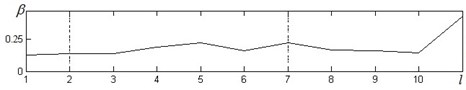
Fig. 6a) inhibitory, b) stationary and c) stimulant processes and their fluctuations in JT interval dynamic during bicycle ergometry test. The test was performed in eleven minutes where 1 minute represented rest interval, 2-6 the load minutes and 6-11 were the interval of recovery of the test (x-axes)

a)

b)

c)

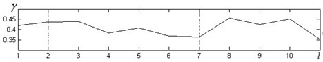
Fig. 7a) inhibitory, b) stationary and c) stimulant processes and their fluctuations in QRS interval dynamic during bicycle ergometry test. The test was performed in eleven minutes where 1 minute represented rest interval, 2-6 the load minutes and 6-11 were the interval of recovery of the test (x-axes)

a)

b)

c)

Another interesting finding related to complexity of ECG intervals RR, JT and QRS is the delay in recovery processes. In the first minute of recovery RR interval shows contrary situation of influencing process – stimulant processes rapidly increase (Fig. 5(c) from 6-th to 7-th minute) while inhibitory process reacts (Fig. 5(a) from 6-th to 7-th minute) to opposite direction. For JT and QRS intervals it is clear expressed delay of stimulant processes in recovery interval (Fig. 6(c), Fig. 7(c) 7-th to 8-th minute). It can illustrate that recovery processes are not synchronous in different human body systems.

Stationary processes (Fig. 5(b), Fig. 6(b), Fig. 7(b)) vary insignificantly during the load and the first four minutes of recovery. It suddenly goes up and reaches its highest value at the last minute of recovery becoming the predominant process influencing the RR, JT and QRS intervals dynamic. This fact may confirm that the recovery processes are over.

5. Conclusions

In analysis of medical or biological investigations it is important to separate data sequences into intervals where similar physiological situations could be observed. In living human body changes of physiological conditions could be very quick and application of statistical technologies or Fourier transform analysis is not always possible. Proposed algebraic analysis could be a technology which can help in analysis of short intervals of data which allows revealing of intervals with stable or unstable physiological features.

In this paper we proposed an algebraic algorithm based on the identification of algebraic progression of sequence of each segment of ECG data.

The human organism could be comprehensible as a complex system that reacts to physical load. The proposed analysis of reactions to physical load could single out different behavior in fluctuations of ECG parameters in different fractal levels.

In case muscles start to monopolize the organism functions, especially during the maximum loads, the suppressive processes became dominant. Increase in stationary processes could reveal the end of recovery processes after the load.

The practical experience has shown that the proposed algebraic algorithm can be effectively used for the analysis of ECG parameters although ECG signals are contaminated with noise.