The dynamic stability of a stepped cantilever beam with attachments

Sochacki, Wojciech

Journal of Vibroengineering

Browse Journal

Submit article

Published: 31 March 2013

Check for updates

The dynamic stability of a stepped cantilever beam with attachments

Wojciech Sochacki¹

¹Częstochowa University of Technology, Institute of Mechanics and Machine Design Foundations, Dąbrowskiego 73, 42-200 Częstochowa, Poland

Cite the article Download PDF

Downloads 1005

WoS Core Citations 10

Abstract

In this paper the problem of the dynamic stability of a stepped cantilever beam with additional discrete elements was investigated. The problem was solved by applying the mode summation method. The influence of the individual discrete elements as well as their locations along the beam on the possibility of a loss in dynamic stability by the investigated system was discussed. The considered beam was treated as an Euler- Bernoulli beam.

1. Introduction

Scientists’ interest in the stepped cantilever beam is dictated by the variety of its application in multiple engineering constructions. A stepped beam of this type can be found in structural building construction, different types of booms, cranes, masts, robots and manipulators. The above mentioned applications are often equipped with different additional elements which influence the dynamics of the whole system. The different axial loads in these types of applications can additionally lead to a significant increase in the amplitude in the cross-sectional oscillations and increase the risk of a loss in dynamic stability. Many works dealing with the dynamic stability of beams with additional discrete elements and with step changes in the cross-section can be found in the literature. Aldraihem and Baz [1] considered the dynamic stability of beams with step changes in the cross-section under moving loads. The dynamic stability of an elastic beam was analysed by Cederbaum and Mond [2]. Chen and Yeh [3] analysed the parametric instability of an electromagnetically excited beam. The same authors [4] studied the dynamic instability of a column carrying a concentrated mass with oscillating motion along the column axis. Evensen and Evan-Iwanowski [5] carried out analytical and experimental research into the influence of a mass mounted at the end of a beam on the dynamic stability of the beam. Gürgöze [6] analysed the influence of a mass mounted at the end of a beam elastically supported along its axis. Hyun and Yoo [7] studied the dynamic stability of an axially oscillating cantilever beam by taking into consideration the stiffness variation. Majorana and Pellegrino [8] analysed the dynamic stability of an elastically supported beam (rotation and translation springs at the ends). Kar and Sujata [9] studied the parametric instability region of a cantilever beam subjected to a time-dependent axial force. The parametric instability regions of a cantilever beam with tip mass subjected to a time-varying magnetic ﬁeld and axial force were analysed by Pratiher and Dwivedy [10]. Sato et al. [11] investigated the parametric vibrations of a horizontal beam loaded by a concentrated mass, which showed the influence of the beam weight and the inertia of a rotational mass on the beam vibrations. Sochacki [12] investigated a simply supported beam axially loaded by a harmonic force, showing the destabilising effect of the concentrated mass, spring and harmonic oscillator.

This paper considers a stepped cantilever beam loaded by a longitudinal force in the form $P (t) = P_{0} + S \cos (ν t)$ . Additionally, a mass, a translational and rotational spring and a discrete element with rotary inertia were connected to the beam at a chosen position between the supports. A change in the cross-section was made at a selected place on the beam length. Additionally, the undamped harmonic oscillator can be attached at a point where the cross-section of the beam changes. The considered beam was treated as a Bernoulli – Euler beam. The problem of dynamic stability was solved using the mode summation method. The applied research procedure allowed the dynamics of the tested system to be described with the use of the Mathieu equation in the form $\ddot{T} (τ) + (a + b c o s τ) T (τ) = 0$ . The influence of the additional mass, translational and rotational springs, the rotary inertia of the discrete element and the undamped harmonic oscillator and their positions on the beam on the value of coefficient $b$ in the Mathieu equation was investigated. Similarly, the influence of step changes in the cross-section of the beam and its position along the beam length on the value of coefficient $b$ was investigated. In this way the possibility of a loss of dynamic stability by the investigated systems was determined.

2. Mathematical model of beam vibrations

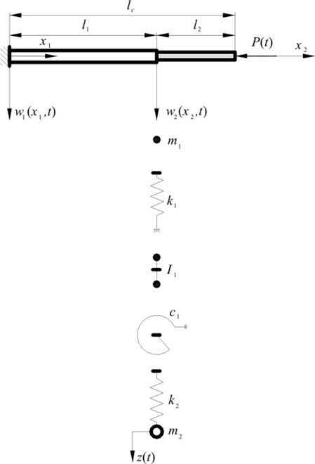
A diagram of the considered beam is presented in Fig. 1.

The vibration equation for two parts of the beam is known and has the following form:

1

E_{i} J_{i} \frac{\partial^{4} w_{i} (x_{i}, t)}{\partial x_{i}^{4}} + P (t) \frac{\partial^{2} w_{i} (x_{i}, t)}{\partial x_{i}^{2}} + ρ_{i} A_{i} \frac{\partial^{2} w_{i} (x_{i}, t)}{\partial t^{2}} = 0,

where: $P (t) = P_{0} + S \cos (ν t)$ , $ν$ – forcing frequency, $ρ_{i}$ – density, $A_{i}$ – cross-section area, $i =$ 1, 2 – $i$ th part of the beam.

The geometrical boundary conditions, continuity condition as well as natural boundary and matching conditions, where the discrete elements are attached, are as follows:

2

w_{1} (0, t) = 0,

{\frac{\partial w_{1} (0, t)}{\partial x_{1}}|}_{x_{1} = 0} = 0,

w_{1} (l_{1}, t) = w_{2} (0, t),

{\frac{\partial w_{1} (x_{1}, t)}{\partial x_{1}}|}^{x_{1} = l_{1}} = {\frac{\partial w_{2} (x_{2}, t)}{\partial x_{2}}|}_{x_{2} = 0},

E_{1} J_{1} {\frac{\partial^{2} w_{1} (x_{1}, t)}{\partial x_{1}^{2}}|}^{x_{1} = l_{1}} + c_{1} {\frac{\partial w_{1} (x_{1}, t)}{\partial x_{1}}|}^{x_{1} = l_{1}} - E_{2} J_{2} {\frac{\partial^{2} w_{1} (x_{2}, t)}{\partial x_{2}^{2}}|}_{x_{2} = 0} = I_{1} {\frac{\partial^{3} w_{1} (x_{1}, t)}{\partial x_{1} \partial t^{2}}|}^{x_{1} = l_{1}},

E_{2} J_{2} {\frac{\partial^{2} w_{2} (x_{2}, t)}{\partial x_{2}^{2}}|}^{x_{2} = l_{2}} = 0,

E_{2} J_{2} {\frac{\partial^{3} w_{2} (x_{2}, t)}{\partial x_{2}^{3}}|}^{x_{2} = l_{2}} + P (t) {\frac{\partial w_{2} (x_{2}, t)}{\partial x_{2}}|}^{x_{2} = l_{2}} = 0,

{E_{1} J_{1} \frac{\partial^{3} w_{1} (x_{1}, t)}{\partial x_{1}^{3}}|}^{x_{1} = l_{1}} + P (t) {\frac{\partial w_{1} (x_{1}, t)}{\partial x_{1}}|}^{x_{1} = l_{1}} - k_{1} w_{1} (l_{1}, t) - m_{1} {\frac{\partial^{2} w_{1} (x_{1}, t)}{\partial t^{2}}|}^{x_{1} = l_{1}} - k_{2} [z (t) - w_{1} (l_{1}, t)] - E_{2} J_{2} {\frac{\partial^{3} w_{2} (x_{2}, t)}{\partial x_{2}^{3}}|}_{x_{2} = 0} - P (t) {\frac{\partial w_{2} (x_{2}, t)}{\partial x_{2}}|}_{x_{2} = 0} = 0,

m_{2} \frac{\partial^{2} z (t)}{\partial t^{2}} + k_{2} [z (t) - w_{1} (l_{1}, t)] = 0 .

During the vibrations, the displacement of the beam and oscillator mass takes the form:

3

w_{i} (x_{i}, t) = W_{i} (x_{i}) c o s (ω t), (i = 1, 2),

4

z (t) = Z c o s (ω t),

where $W_{i} (x_{i})$ and $Z$ are displacement amplitudes $w$ and $z$ , while $ω$ is the natural frequency of the cantilever stepped beam with discrete elements.

Fig. 1Model of the beam with step changes in the cross-section with additional discrete elements

Substituting (3) and (4) into equations (1) and into conditions (2) one can obtain (for $S = 0$ ):

5

E_{i} J_{i} W_{i}^{I V} (x_{i}) + P_{0} W_{i}^{I I} (x_{i}) - ρ_{i} A_{i} ω^{2} W_{i} (x_{i}) = 0, (i = 1, 2),

and:

6

W_{1} (0) = 0, W_{1}^{I} (0) = 0,

E_{2} J_{2} W_{2}^{I I} (l_{2}) = 0, E_{2} J_{2} W_{2}^{I I I} (l_{2}) + P_{0} W_{2}^{I} (l_{2}) = 0,

E_{1} J_{1} W_{1}^{I I I} (l_{1}) + (m_{1} ω^{2} - k_{1}) W_{1} (l_{1}) + m_{2} ω^{2} Z - E_{2} J_{2} W_{2}^{I I I} (0) = 0,

W_{1} (l_{1}) = W_{2} (0), W_{1}^{I} (l_{1}) = W_{2}^{I} (0),

E_{1} J_{1} W_{1}^{I I} (l_{1}) + c_{1} W_{1}^{I} (l_{1}) - E_{2} J_{2} W_{2}^{I I} (0) = I_{1} ω^{2} W_{1}^{I} (l_{1}),

k_{2} (Z - W_{1} (l_{1})) - m_{2} ω^{2} Z = 0,

where the Roman numerals denote differentiation with respect to $x$ .

The general solution to equations (5) takes the form:

7

W_{i} (x_{i}) = C_{i 1} c o s h (α_{i} x_{i}) + C_{i 2} s i n h (α_{i} x_{i}) + C_{i 3} c o s (β_{i} x_{i}) + C_{i 4} s i n (β_{i} x_{i}),

where $C_{i k}$ are constants ( $k =$ 1, 2, 3, 4) and:

8

α_{i}^{2} = - \frac{λ_{i}}{2} + \sqrt{\frac{λ_{i}^{2}}{4} + Ω_{i}}, β_{i}^{2} = \frac{λ_{i}}{2} + \sqrt{\frac{λ_{i}^{2}}{4} + Ω_{i}},

where: $Ω_{i}^{2} = ω^{2} \frac{ρ_{i} A_{i}}{E_{i} J_{i}}$ , $λ_{i} = \frac{P_{0}}{E_{i} J_{i}}$ , $i =$ 1, 2.

The equations of vibrations (5) together with the boundary conditions (6) allow the boundary value problem of the investigated beam to be formulated. The natural frequency $ω$ and eigenfunctions of the beam $W_{i} (x_{i})$ are determined by solving the boundary value problem.

After substituting equations (7) into (6), one obtains a system of nine homogenous equations for the unknown constants $C_{i k}$ , which can be written in matrix form as:

9

[A] (ω) C = 0,

where: $A (ω) = [a_{p q}]$ , ( $p, q =$ 1, 2, …, 9) and $C = {[C_{11} . . . C_{14}, C_{21} . . . C_{24}, Z]}^{T}$ .

For a non-trivial solution to equation (9), the determinant of the matrix $A (ω)$ is set equal to zero, yielding the frequency equation:

10

det A (ω) = 0 .

The non-zero elements $a_{p q}$ of matrix $A (ω)$ are given as follows:

11

a_{11} = 1, a_{13} = 1,

a_{22} = a_{1}, a_{24} = β_{1},

a_{31} = α_{1} \sinh (α_{1}^{*}), a_{23} = α_{1} \cosh (α_{1}^{*}), a_{33} = - β_{1} \sin (β_{1}^{*}),

a_{34} = β_{1} \cos (β_{1}^{*}), a_{36} = - α_{1}, a_{38} = - β_{2},

a_{41} = \cosh (α_{1}^{*}), a_{42} = \sinh (α_{1}^{*}), a_{43} = \cos (β_{1}^{*}), a_{44} = \sin (β_{1}^{*}), a_{45} = - 1, a_{47} = - 1,

a_{51} = E_{1}^{*} α_{1}^{2} c o s h (α_{1}^{*}) + c_{1} α_{1} s i n h (α_{1}^{*}) - ω^{2} I_{1} α_{1} s i n h (α_{1}^{*}),

a_{52} = E_{1}^{*} α_{1}^{2} s i n h (α_{1}^{*}) + c_{1} α_{1} c o s h (α_{1}^{*}) - ω^{2} I_{1} α_{1} c o s h (α_{1}^{*}),

a_{53} = - E_{1}^{*} β_{1}^{2} c o s (β_{1}^{*}) - c_{1} β_{1} s i n (β_{1}^{*}) + ω^{2} I_{1} β_{1} s i n (β_{1}^{*}),

a_{54} = - E_{1}^{*} β_{1}^{2} s i n (β_{1}^{*}) + c_{1} β_{1} c o s (β_{1}^{*}) - ω^{2} I_{1} β_{1} c o s (β_{1}^{*}),

a_{55} = - E_{2}^{*} α_{2}^{2}, a_{57} = E_{2}^{*} β_{2}^{2},

a_{65} = E_{2}^{*} α_{2}^{2} c o s h (α_{2}^{*}), a_{66} = E_{2}^{*} α_{2}^{2} s i n h (α_{2}^{*}),

a_{67} = - E_{2}^{*} β_{2}^{2} c o s (β_{2}^{*}), a_{68} = - E_{2}^{*} β_{2}^{2} s i n (β_{2}^{*}),

a_{75} = E_{2}^{*} α_{2}^{3} s i n h (α_{2}^{*}) + P_{0} α_{2} s i n h (α_{2}^{*}), a_{76} = E_{2}^{*} α_{2}^{3} c o s h (α_{2}^{*}) + P_{0} α_{2} c o s h (α_{2}^{*}),

a_{77} = E_{2}^{*} β_{2}^{3} s i n (β_{2}^{*}) - P_{0} β_{2} s i n (β_{2}^{*}), a_{78} = - E_{2}^{*} β_{2}^{3} c o s (β_{2}^{*}) + P_{0} β_{2} c o s (β_{2}^{*}),

a_{81} = E_{1}^{*} α_{1}^{3} s i n h (α_{1}^{*}) - (k_{1} - ω^{2} m_{1}) c o s h (α_{1}^{*}),

a_{82} = E_{1}^{*} α_{1}^{3} c o s h (α_{1}^{*}) - (k_{1} - ω^{2} m_{1}) s i n h (α_{1}^{*}),

a_{83} = E_{1}^{*} β_{1}^{3} s i n (β_{1}^{*}) - (k_{1} - ω^{2} m_{1}) c o s (β_{1}^{*}),

a_{84} = - E_{1}^{*} β_{1}^{3} c o s (β_{1}^{*}) - (k_{1} - ω^{2} m_{1}) s i n (β_{1}^{*}),

a_{86} = - E_{2}^{*} α_{2}^{3}, a_{88} = E_{2}^{*} β_{2}^{3}, a_{89} = ω^{2} m_{2},

a_{91} = k_{2} \cosh (α_{1}^{*}), a_{92} = - k_{2} \sinh (α_{1}^{*}), a_{93} = - k_{2} \cos (β_{1}^{*}),

a_{94} = - k_{2} s i n (β_{1}^{*}), a_{99} = k_{2} - ω^{2} m_{2},

where: $α_{i}^{*} = α_{i} l_{i}$ , $β_{1}^{*} = β_{i} l_{i}$ , $E_{i}^{*} = E_{i} J_{i}$ , $i = 1,2$ .

3. The solution to the problem of the dynamic stability of the beam

The solution to equation (1) is assumed to be in the form of eigenfunction series:

12

w_{i} (x_{i}, t) = \sum_{n = 1}^{\infty} W_{i n} (x_{i}) T_{n} (t),

where $T_{n} (t)$ are unknown time functions and $W_{i n} (x_{i})$ are the normalized eigenfunctions of the free frequencies of $i$ -th parts of the beam which satisfies:

13

\sum_{i = 1}^{2} ρ_{i}^{*} \int_{0}^{l_{i}} W_{i n} (x_{i}) W_{i m} (x_{i}) d x_{i} + I_{1} W_{1 n}^{I} (l_{1}) W_{1 m}^{I} (l_{1}) + {W_{1 m} (l_{1}) W_{1 n} (l_{1}) (m_{1} + m_{2} \frac{k_{2}^{2}}{(k_{2} - m_{2} ω_{m}^{2}) (k_{2} - m_{2} ω_{n}^{2})})|}_{= γ_{m}^{2} f o r m = n,}^{= 0 f o r m \neq n,}

where: $γ_{m}^{2} = \sum_{i = 1}^{2} ρ_{i}^{*} \int_{0}^{l_{i}} W_{i m}^{2} (x_{i}) d x_{i} + I_{1} {W_{1 m}^{I}}^{2} (l_{1}) + (m_{1} + m_{2} \frac{k_{2}^{2}}{{(k_{2} - m_{2} ω_{m}^{2})}^{2}}) W_{1 m}^{2} (l_{1})$ and $ρ_{i}^{*} = ρ_{i} A_{i}$ , $i =$ 1, 2.

Substituting solutions (12) into equation (1) one can obtain:

14

\sum_{n = 1}^{\infty} [E_{i} J_{i} W_{i n}^{I V} (x_{i}) T_{i n} (t) + (P_{0} + S c o s ν t) W_{i n}^{I I} (x_{i}) T_{i n} (t) + ρ_{i} A_{i} W_{i n} (x_{i}) {\ddot{T}}_{i n} (t)] = 0 .

After multiplying by $W_{i m} (x_{i})$ , one can receive:

15

\sum_{n = 1}^{\infty} [E_{i} J_{i} W_{i n}^{I V} (x_{i}) W_{i m} (x_{i}) T_{n} (t) + P_{0} W_{i n}^{I I} (x_{i}) W_{i m} (x_{i}) T_{n} (t) + S c o s ν t W_{i n}^{I I} (x_{i}) W_{i m} (x_{i}) T_{n} (t) + ρ_{i} A_{i} W_{i n} (x_{i}) W_{i m} (x_{i}) {\ddot{T}}_{n} (t)] = 0 .

By analogy, from equations (5), after multiplying by $W_{i m} (x_{i})$ , one can obtain:

16

E_{i} J_{i} W_{i n}^{I V} (x_{i}) W_{i m} (x_{i}) + P_{0} W_{i n}^{I I} (x_{i}) W_{i m} (x_{i}) = ρ_{i} A_{i} ω_{n}^{2} W_{i n} (x_{i}) W_{i m} (x_{i}), (i = 1, 2),

then (15) takes the following form:

17

\sum_{n = 1}^{\infty} [ρ_{i} A_{i} ω_{n}^{2} W_{i n} (x_{i}) W_{i m} (x_{i}) T_{n} (t) + S c o s ν t W_{i n}^{I I} (x_{i}) W_{i m} (x_{i}) T_{n} (t) + ρ_{i} A_{i} W_{i n} (x_{i}) W_{i m} (x_{i}) {\ddot{T}}_{n} (t)] = 0 .

As only the basic parametric resonance with the first natural frequency of the beam is taken into account in this paper, further analysis considers the first term of the sum from equations (12). Hence, after integrating equations (17), the following form was obtained for the whole beam and the first term:

18

T_{1} (t) (ω_{1}^{2} ρ_{i} A_{i} \int_{0}^{l} W_{i 1}^{2} (x_{i}) d x_{i} + S c o s ν t \int_{0}^{l} W_{i 1}^{I I} (x_{i}) W_{i 1} (x_{i}) d x_{i}) + {\ddot{T}}_{1} (t) ρ_{i} A_{i} \int_{0}^{l} W_{i 1}^{2} (x_{i}) d x_{i} = 0 .

Appropriate transformations of equation (18) and the substitution of $t$ by a new variable $τ = ν t$ lead to the following form of the Mathieu equation:

19

\ddot{T} (τ) + (a + b c o s τ) T (τ) = 0,

where: $a = \frac{ω_{1}^{2}}{ν^{2}}$ , $b = \frac{S}{ν^{2}} \frac{\sum_{i = 1}^{2} \int_{0}^{l} W_{i 1}^{I I} (x_{i}) W_{i 1} (x_{i}) d x_{i}}{\sum_{i = 1}^{2} ρ_{i} A_{i} \int_{0}^{l} W_{i 1}^{2} (x_{i}) d x_{i}}$ , dots denote differentiation with respect to $τ$ .

The periodical solutions to the Mathieu equation (19) are known as the Strutt’s card (see: Timoshenko and Gere [13]). These solutions allow us to determine the stable and unstable regions of the solutions. The numerical values of $a$ and $b$ each time determined whether the position of the solution is in the stable or unstable region. However, it must be stated that the probability of obtaining a stable solution is higher in the case of a lower value of coefficient $b$ , at the determined value of $a$ . On the stability card, coefficient $b$ takes positive and negative values symmetrically in relation to axis $a$ for $b =$ 0. In this paper the analysis of changes in coefficient $b$ was carried out assuming $b = | - b |$ . In the mathematical model of vibrations of the stepped cantilever beam, the influence of damping on the dynamic stability of the tested system has been omitted. Consideration of damping leads to constraint of the regions of the stable solutions in the Strutt’s card. Then, a loss in the dynamic stability takes place for the higher values of parameter $b$ .

4. The results of numerical computations

Computations were carried out assuming the following dimensionless quantities:

20

K_{1} = \frac{k_{1} l_{c}^{3}}{E_{1} J_{1}}, K_{2} = \frac{k_{2} l_{c}^{3}}{E_{1} J_{1}}, C_{1} = \frac{c_{1} l_{c}}{E_{1} J_{1}}, I = \frac{A_{1} l_{c}^{2}}{I_{1}}, J = \frac{J_{2}}{J_{1}},

M_{1} = \frac{m_{1}}{\sum_{i = 1}^{2} ρ_{i} A_{i} l_{i}}, M_{2} = \frac{m_{2}}{\sum_{i = 1}^{2} ρ_{i} A_{i} l_{i}}, l = \frac{l_{1}}{l_{c}}, p = \frac{P_{0}}{P_{c}}, s = \frac{S}{P_{c}},

where $P_{c}$ – the critical load of the tested beam with a constant cross-section.

The final results of the tests were selected to represent the correlation between the size of the descrete element (change in the value of the specific size characteristic for this element), as well as the influence of a change in the location of the attachment point for the same element along the beam length on the values of coefficient $b$ in the Mathieu equation. Computations were performed for the following data: $p =$ 0.05, $s =$ 0.05, $a =$ 1.085.

The influence of an increase in the characteristic quantity for an element attached to the beam in relation to its dynamic stability is presented in Figures 2-7. The final results were acquired when the descrete element was attached to the beam within a distance of $l =$ 0.2 (at the point where the cross-section changes and in the case of the element with rotary inertia). In all other cases, the discrete element was attached to the beam within a distance of $l =$ 0.8.

In the Strutt’s card, the point of data $(a, b)$ is a picture of the solution to equation (19) for a system with specified physical and geometrical data and a specific frequency of an exciting force. Exemplary results of research into the system, presented in Figs. 2-7 in the form of straight lines, come from the changes in the frequency of the exciting force.

Fig. 2Exemplary positions of solutions to the Mathieu equation (19) for chosen values of mass M1: M1= 1 , M1= 0.6 , M1= 0.2.

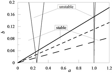
Fig. 3Exemplary positions of solutions to the Mathieu equation (19) for chosen values of elasticity coefficient K1: K1= 100 , K1= 20 , K1= 10

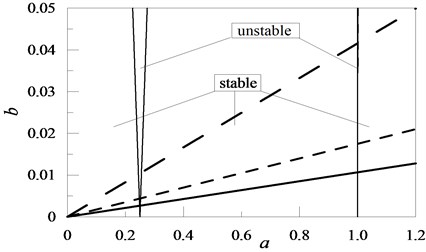
Fig. 4Exemplary positions of solutions to the Mathieu equation (19) for chosen values of I: I= 2 , I= 1 , I= 0.1

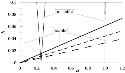
Fig. 5Exemplary positions of solutions to the Mathieu equation (19) for chosen values of C1: C1= 100 , C1= 10 , C1= 1

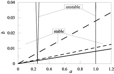
Fig. 6Exemplary positions of solutions to the Mathieu equation (19) for chosen values of the elasticity coefficient of oscillator K2 for M2= 0.2: K2= 10 , K2= 2 , K2= 1

Exemplary positions of solutions to the Mathieu equation (19) for chosen values of the elasticity coefficient of oscillator K2 for M2= 0.2: K2= 10 , K2= 2 , K2= 1

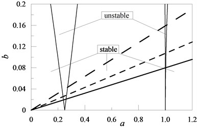
Fig. 7Exemplary positions of solutions to the Mathieu equation (19) for chosen values of relations J: J= 0.5 , J= 0.2 , J= 0.1.

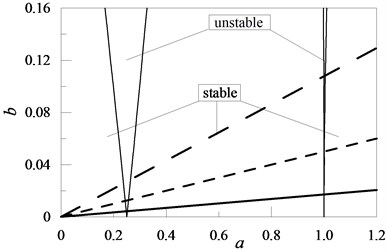
Fig. 8The influence of the mounted position of mass M1 on the beam and its values on the value of coefficient b for M1= 1 , M1= 0.6 , M1= 0.2

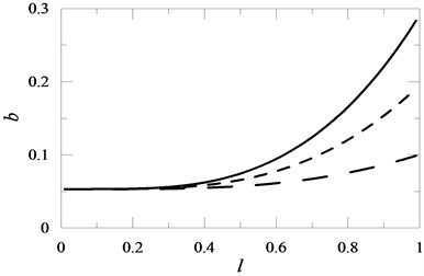
Fig. 9The influence of the position of a translational spring with elasticity coefficient K1 mounted on the beam on the value of coefficient b for K1= 20 , K1= 10 , K1= 1

The influence of the position of a translational spring with elasticity coefficient K1 mounted on the beam on the value of coefficient b for K1= 20 , K1= 10 , K1= 1

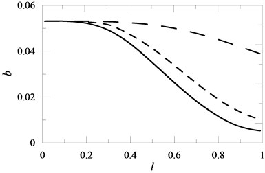
Fig. 10The influence of the position of an element with rotary inertia I mounted on the beam on the value of coefficient b for I= 2 , I= 1 , I= 0.1

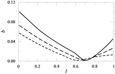
Fig. 11The influence of the position of a rotational spring with elasticity coefficient C1 mounted on the beam on the value of coefficient b for C1= 100 , C1= 10 , C1= 1.

The influence of the position of a rotational spring with elasticity coefficient C1 mounted on the beam on the value of coefficient b for C1= 100 , C1= 10 , C1= 1.

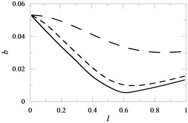
Fig. 12The influence of the oscillator mounting location on the beam and the value of the elasticity coefficient K2 on the value of coefficient b for M2= 0.2: K2= 1 , K2= 2 , K2= 10

The influence of the oscillator mounting location on the beam and the value of the elasticity coefficient K2 on the value of coefficient b for M2= 0.2: K2= 1 , K2= 2 , K2= 10

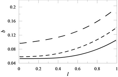
Fig. 13The influence of the location of changes in the cross-section l of the beam on the value of coefficient b in the Mathieu equation for J= 0.5 , J= 0.2 , J= 0.1

The influence of the location of changes in the cross-section l of the beam on the value of coefficient b in the Mathieu equation for J= 0.5 , J= 0.2 , J= 0.1

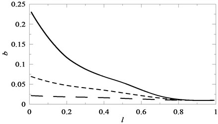
The influence of the location of the attached discrete element along the beam length on the value of coefficient $b$ in the Mathieu equation is shown in the next set of figures (Figs. 8-13). The values, characteristic for each of the discrete elements, were changed in the same way as in the case of the tests whose final results were presented in Figs. 2-7.

5. Conclusions

The formulation and solution to the problem of the dynamic stability of a stepped cantilever beam with attached additional discrete elements was presented in the paper. The value of coefficient $b$ in the Mathieu equation (19) was assumed as the possibility of a loss in dynamic stability by the beam. Analysis of the influence of individual discrete elements on the dynamic stability of the tested system was carried out on the basis of the formulation of and solution to the problem.

Analysing the presented research results one can notice, that in the case of the cantilever beam, an increase in the attached concentrated mass as well as the moment of inertia $I$ of the element with rotational inertia (Figs. 2, 4) is disadvantageous. In these cases, the attachment of the given element in an optional location along the beam length caused an increase in the value of coefficient $b$ in the Mathieu equation. An increase in the values of the characteristic quantities for the remaining discrete elements resulted in the stability of the system (a decrease in the value of coefficient $b$ – Figs. 3, 5, 6 and 7).

Analysis of the influence of the attachment point of a given discrete element to the beam on its dynamic stability allowed the following statements to be formulated.

In the case of concentrated mass (Fig. 8), the most disadvantageous position was its attachment at the free end of the beam. The location of the attachment point of the element with rotational inertia to the beam had an essential influence on its stability. The system was stabilised, reaching minimal value $b$ in dependence on value $I$ , when the distance from the restrain place was increased. A further increase in distance $l$ caused the destabilisation of the system (Fig. 10). Similarly, the position of a rotational spring with elasticity coefficient $C_{1}$ (Fig. 11) influenced the dynamic stability of the system. But in this case, the system was stabilised, reaching minimal value $b$ at the free end of the beam for the small value of $C_{1} (C_{1} = 1)$ with an increase in $l$ .

Attaching a translational spring (Fig. 9) to the beam unequivocally influenced the stability of the system cantilever beam – discrete element. Assuming the same elasticity coefficient $K_{1}$ , higher stabilisation was obtained with an increase in parameter $l$ . Parameter $l$ characterised the distance between the spring clamping and the point of beam restraint. Similar stability was obtained by an increase in the elasticity coefficient of the spring of the harmonic oscillator attached to cantilever beam $K_{2}$ . In this case, for a constant value of coefficient $K_{2}$ , the tested system was less stable the further the location of the oscillator from the point of beam restraint (Fig. 12). This was connected to the fact that the research was carried out for a constant value of oscillator mass which destabilized the tested system. Modification of the point of change in the beam cross-section and modification of this change (increase in coefficient $J$ ) stabilized the tested system. In this case it was obvious because a change in the point of the beam cross-section was connected to a simultaneous increase in the length of the beam with a higher cross-section (Fig. 13).

6.

References

Aldraihem O. J., Baz A. Dynamic stability of stepped beams under moving loads. Journal of Sound and Vibration, Vol. 205, Issue 5, 2002, p. 835-848.

Search CrossRef
Cederbaum G., Mond M. Stability properties of a viscoelastic column under a periodic force. Journal of Applied Mechanics, Vol. 59, 1992, p. 16-19.

Search CrossRef
Chen C.-C., Yeh M.-K. Parametric instability of a beam under electromagnetic excitation. Journal of Sound and Vibration, Vol. 240, Issue 4, 2001, p. 747-764.

Search CrossRef
Chen C.-C., Yeh M.-K. Parametric instability of a column with axially oscillating mass. Journal of Sound and Vibration, Vol. 224, Issue 4, 1999, p. 643-664.

Search CrossRef
Evensen H. A., Evan-Iwanowski R. M. Effects of longitudinal inertia upon the parametric response of elastic columns. ASME Journal of Applied Mechanics, Vol. 33, 1966, p. 141-148.

Search CrossRef
Gürgöze M. Parametric vibrations of restrained beam with an end mass under displacement excitation. Journal of Sound and Vibration, Vol. 108, Issue 1, 1986, p. 73-84.

Search CrossRef
Hyun S. H., Yoo H. H. Dynamic modeling and stability analysis of axially oscillating cantilever beams. Journal of Sound and Vibration, Vol. 228, Issue 3, 1999, p. 543-558.

Search CrossRef
Kar R. C., Sujata T. Parametric instability of an elastically restrained cantilever beam. Computers and Structures, Vol. 34, 1990, p. 469-475.

Search CrossRef
Majorana C. E., Pellegrino C. Dynamic stability of elastically constrained beams: an exact approach. Engineering Computations, Vol. 14, Issue 7, 1997, p. 792-805.

Search CrossRef
Pratiher B., Dwivedy S. K. Parametric instability of a cantilever beam with magnetic ﬁeld and periodic axial load. Journal of Sound and Vibration, Vol. 305, Issue 5, 2007, p. 904-917.

Search CrossRef
Sato K., Saito V., Otomi V. The parametric response of a horizontal beam carrying a concetrated mass under gravity. ASME Journal of Applied Mechanics, Vol. 45, 1978, p. 643-648.

Search CrossRef
Sochacki W. The dynamic stability of a simply supported beam with additional discrete elements. Journal of Sound and Vibration, Vol. 314, Issue 1-2, 2008, p. 180-193.

Search CrossRef
Timoshenko S. P.,Gere V. Theory of Elastic Stability. Mc Graw–Hill, Inc., 1961.

Search CrossRef

About this article

Received

30 November 2012

Accepted

28 February 2013

Published

31 March 2013

Keywords

dynamic stability

Mathieu equation

eigenfunctions

stepped beam

Acknowledgements

This research was supported by the Ministry of Science and Higher Education in 2012, Warsaw, Poland.

This is an open access article distributed under the Creative Commons Attribution License, which permits unrestricted use, distribution, and reproduction in any medium, provided the original work is properly cited.