Abstract
This research aims at estimating the life of the beam with normal distribution parameters and subjected to cyclic load. It is tested by Monte-Carlo simulation that the generalized displacement and velocity are normally distributed when the coefficient of variation () of the random parameter is small (generally 0.01). The random perturbation method is employed to estimate the mean and variance of the generalized displacement and velocity. The random dynamic stress and its derivative with respect to the time of the beam is formulated according to the shape function of beam element and the stress equation in a Euler-Bernoulli beam. Their mean, variance and correlation coefficient are given using the first-order approximation in a Taylor series. Based on Palmgren-Miner rule, the expected cumulative damage equation is given and is used to estimate the life where the random dynamic stress is non-stationary and follows the normal distribution with the nonzero mean at any time . The presented method could also estimate the life of other structure or component which has several normal random parameters, is subjected to cyclic load and obeys the linear dynamics and elastic theory when the random parameter’s is small.
1. Introduction
The beam is the common structural element of the civil and mechanical engineering. It could withstand the bending moment and shear force primarily. If the beam failure occurs during service, it should lead to the huge economic lost or the casualties. The failure due to fatigue might be the common one. In mechanical engineering, there are a lot of factors which result in the beam with random parameters. The factors should include manufacturing error of machine tool, ambient temperature, random vibration of the foundation of machine tool, material uniformity and so on. Moreover, many beams used in mechanical engineering commonly carry the cyclic load, such as the loads due to all kinds of faults of the rotating machine. Therefore, it is important to estimate the life of the beam with random parameters and subjected to the cyclic load.
The random parameters of the beam result in the random stress under the deterministic cyclic load. The known methods of estimating the life of metallic structures and components under random stress can be classified into two groups: time-domain method based on a cycle counting method and frequency-domain method using power spectral density (PSD) of stochastic processes [1]. One of time-domain method, the combination of rainflow counting and Palmgren-Miner rule, is recognized as the “gold standard” for estimating fatigue damage from variable amplitude stress or for comparison to other estimate techniques [2, 3]. However, it has been proved to spend a lot of time in processing data when time-domain method is employed to estimate the life under random stress [4, 5]. For the reason, frequency-domain method has been developed. It can produce (exact or approximated) analytical expressions by which we can estimate cycle distribution and fatigue life under a given counting procedure, without, however, requiring knowledge of each stress or strain time history [6, 7]. The life estimation of the beam under random stress has reported by some documents. The focus of the reported works is to predict the life of the beam with the deterministic parameters and withstanding the random loading. For example, the fatigue life prediction method of the dual cantilever beam subjected to the narrow band random load was introduced by Rajnikant Bhogilal Thakkar [8] and was based on the fatigue life under the variable sinusoidal load. The fatigue life of the Aluminum 6061 T6 cantilever beam, where the input was the white noise acceleration, were predicted using seven types of the frequency methods and Rainflow counting method respectively and they were compared with these obtained by experiments in [9]. The effect of the damping ratios of the test structure on the fatigue life was also analyzed by the four types of tests with the different damping ratios. An analytic methodology was developed by Paulus et al. [10] to predict the fatigue life of the cantilever beam experiencing stationary and Gaussian random vibration excitation. In addition, Paulus et al. [11] proposed a semi-empirical life method of the cantilevered beam subjected to the random excitation with a wide range of PSD (power spectral density) shapes and amplitudes. Two methods were employed by Lin et al. [12, 13] to predict the fatigue lives of RC beams strengthened with CFL (carbon fiber laminate) subjected to the exciting force due to the random traffic flow. They were based on the residual life model and the residual strength model respectively. Moreover, the fatigue life of the beam with the uncertain parameters was discussed by a few works. For example, the effect of the uncertainties on the fatigue life of a higher order sandwich beam was discussed by Wang and Sun [14]. In their work, the uncertainties included the density of foam core materials and the thicknesses of the core and the top bottom skins, two independent white noise loadings with the same spectral density function were applied to two different points on the top skin.
It has not been reported to estimate the fatigue life of the beam which has several random parameters and is subjected to cyclic load. Therefore, it should be discussed in this work. Here, these random parameters are assumed to be normally distributed. The remainder of this paper is organized as follows: In Section 2, it should be tested by Monte-Carlo simulation that the generalized displacement and velocity follow normal distributions with the periodic mean and variance estimated by the random perturbation method, and the mean, variance and correlation coefficient of the random dynamic stress and its time derivative are formulated using the first-order approximation in a Taylor series. In Section 3, the expected cumulative damage based on Palmgren-Miner rule is modeled where the random dynamic stress is non-stationary and follows the normal distribution with the nonzero mean at any time . The conclusions are drawn finally.
2. Random dynamical stress analysis of the beam with normal distribution parameters
2.1. Random dynamical response analysis
When the beam undergoes small random vibrations around a position of stable equilibrium and is assumed to be with viscous damping, the dynamical equation of the beam with random parameters is:
where , and are the × dimension mass matrix, damping matrix and stiffness matrix respectively and is the dimension external load vector of which the element is the cyclic external load. , and are the dimension generalized acceleration, velocity and displacement vector respectively. is the total number of the degree of freedom. One or multiple elements of , and are the random variables. All random parameters of the considered beam are written by one random vector . Generally, is composed of the total length , width , height , modulus of elasticity and density which are supposed to be normally distributed and mutually independent. The random perturbation method [15, 16] is employed to analyze the random dynamical response of the dynamical Eq. (1). The mean of the generalized displacement vector is:
where is the deterministic part of the generalized displacement vector and is solved by:
where , and are the deterministic part of , and respectively. They are obtained by substituting the mean of all random parameters into , and . The covariance matrix of the generalized displacement vector is:
where is the sensitivity matrix of to the random vector and is:
is the covariance matrix of the random parameter vector and is:
where is the total number of random parameters and which is solved by:
where is the deterministic part of .
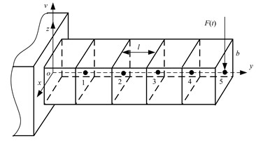
The skewness and kurtosis of the generalized displacement and velocity of node 1, 3 and 5 of the random cantilever beam at 0.005 and 0.012 second are shown in table 1. All random parameters’ is the identical number in one Monte-Carlo simulation. The samples of the generalized displacement are generated by Monte-Carlo method and Newmark- method. The sample size is 5000. The considered cantilever beam with normal distribution parameters is shown in Fig. 1(b). It is divided into 5 elements. The means of the total length , width , height , density and elastic modulus are 0.25 m, 0.02 m, 0.03 m, 7850 kg/m3 and 2.06×10¹¹ Pa respectively. The deterministic cyclic load is applied to the free end node. From Table 1, it could be trusted that the random generalized displacement and velocity at any time are the normal distribution when all CVs of the random parameters are small (generally 0.01).
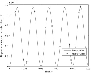
The displacement mean and standard deviation of node 1 of the cantilever beam with normal distribution parameters calculated by Monte-Carlo simulation and random perturbation method respectively with 0.01 are shown in Fig. 2 and 3. Here, the values of the parameters except are identical with the numerical calculation of the skewness and kurtosis of the generalized displacement and velocity. The difference between Monte-Carlo simulation and random perturbation method is very little according to Fig. 2 and 3. In fact, the similar results are found in the mean and standard deviation of the generalized displacement and velocity of other nodes. Therefore, it might be one solution to estimating the mean and variance by random perturbation method when the random generalized displacement and velocity of the beam with normal distribution parameters are normally distributed at any time.
Table 1Skewness and kurtosis of generalized displacement and velocity of node 1, 3 and 5 of cantilever beam with normal distribution random parameters at 0.005 and 0.012 second
Time (s) | Node 1 | Node 3 | Node 5 | |||||||||||
0.005 | 0.005 | Skewness | 0.060 | 0.072 | 0.057 | 0.067 | 0.060 | 0.071 | 0.057 | 0.066 | 0.060 | 0.071 | 0.057 | 0.066 |
Kurtosis | 3.007 | 3.010 | 3.004 | 3.007 | 3.007 | 3.009 | 3.004 | 3.007 | 3.007 | 3.009 | 3.004 | 3.007 | ||
0.012 | Skewness | 0.063 | –0.053 | 0.059 | 0.052 | 0.062 | –0.054 | 0.059 | –0.052 | 0.062 | –0.054 | 0.059 | –0.053 | |
Kurtosis | 3.007 | 3.006 | 3.005 | 3.003 | 3.007 | 3.006 | 3.005 | 3.003 | 3.007 | 3.006 | 3.005 | 3.003 | ||
0.010 | 0.005 | Skewness | 0.148 | 0.171 | 0.145 | 0.168 | 0.148 | 0.170 | 0.145 | 0.166 | 0.148 | 0.169 | 0.145 | 0.165 |
Kurtosis | 3.019 | 3.027 | 3.073 | 3.070 | 3.019 | 3.027 | 3.073 | 3.070 | 3.019 | 3.026 | 3.073 | 3.070 | ||
0.012 | Skewness | 0.153 | –0.135 | 0.150 | –0.131 | 0.153 | –0.136 | 0.150 | -0.132 | 0.153 | –0.137 | 0.149 | –0.134 | |
Kurtosis | 3.021 | 3.017 | 3.072 | 3.084 | 3.020 | 3.017 | 3.073 | 3.082 | 3.020 | 3.017 | 3.073 | 3.081 | ||
0.050 | 0.005 | Skewness | 0.744 | 0.882 | 0.712 | 0.834 | 0.744 | 0.876 | 0.713 | 0.825 | 0.744 | 0.870 | 0.713 | 0.817 |
Kurtosis | 4.138 | 4.541 | 4.056 | 4.413 | 4.134 | 4.522 | 4.057 | 4.383 | 4.135 | 4.563 | 4.058 | 4.362 | ||
0.012 | Skewness | 0.776 | –0.681 | 0.740 | –0.662 | 0.775 | –0.686 | 0.738 | -0.668 | 0.773 | –0.690 | 0.737 | –0.673 | |
Kurtosis | 4.229 | 3.999 | 4.140 | 3.936 | 4.225 | 4.009 | 4.133 | 3.952 | 4.220 | 4.019 | 4.128 | 3.963 | ||
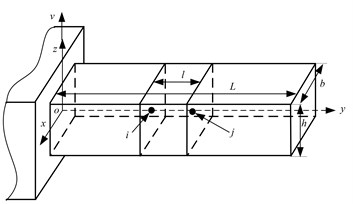
Fig. 1a) Coordinate system and b) finite element model of the beam
a)
b)
Fig. 2Displacement mean of node 1 of the considered cantilever beam with CV= 0.01
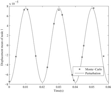
Fig. 3Displacement standard deviation of node 1 of the considered cantilever beam with CV= 0.01
2.2. Random dynamical stress analysis
The coordinate system of the considered beam is shown in Fig. 1(a). The normal stress of a cross-section of the Euler-Bernoulli beam for the application of bending moment and transverse force is [17]:
where is the axial direction coordinate of the cross-section, is the bending moment of the cross-section at the time , is area moment of inertia and is the distance to neutral axis of the cross-section. By substituting the approximate differential equation of the deflection curve of the beam into Eq. (8), the normal stress is:
where , are the modulus of elasticity and the deflection of the cross-section at the time respectively. The maximal normal stress of the cross-section at the time is:
In the finite element method for the Euler-Bernoulli beam, between any two adjacent node and (, 1, 2, 3,…, and ) is:
where the -coordinate of the node is more than that of the node , , , and are the lateral displacement and rotation of the node and respectively and is the element length. According to Eq. (11), the maximal normal stress of the cross-section at the time is normally distributed if , , and are normally distributed. Then, by expanding the maximal normal stress of the cross-section to first-order approximation in a Taylor series at a point , the mean and variance are respectively calculated by [18]:
where:
is vector and:
According to the random perturbation method and Eq. (10) and (11), the partial derivative of the maximal normal stress of the cross-section with respect to the random variable (1, 2,…, ) between any two adjacent node and :
where and .
By combining Eqs. (10) and (11), the time derivative of the maximal normal stress of the cross-section is:
Then, its approximate mean and variance could be calculated by Eqs. (12-14) where is replaced by and . According to Eq. (16), the time derivative of the maximal normal stress of the cross-section at the time is normally distributed if , , and are normally distributed. By expanding the maximal normal stress of the cross-section and its time derivative to first-order approximation in a Taylor series at a point and respectively are:
where and are the mean of the random variables and respectively. Then, the correlation coefficient between and is:
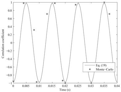
The mean and standard deviation of the maximal fixed-end stress of the cantilever beam calculated using the presented method are compared with these by Monte-Carlo simulation in Fig. 4 and 5 respectively. The correlation coefficient between the maximal fixed-end stress and its time derivative calculated by Monte-Carlo simulation and Eq. (19) is shown in Fig. 6. Here, 0.005 and other parameters are the same as Section 2.1. It could be seen that the mean, standard deviation and correlation coefficient estimated by the presented method are very close to these calculated by Monte-Carlo simulation from Figs. 4, 5 and 6. In fact, there is only a small difference between the mean, standard deviation and correlation coefficient estimated by the presented method and Monte-Carlo simulation when of all random parameters is less than about 0.01.
3. Life estimation of a beam with normal distribution parameters and subjected to cyclic load
According to Palmgren-Miner rule, the expected cumulative damage during the time interval to is [19]:
where and are constants depending on the material, and are replaced by and respectively for simplicity, is the expected number of crossings (at level , with positive slope) and is calculated by [20]:
If and are normally distributed, their joint probability density function is:
where is estimated by Eq. (19), and . Then, the expected number of crossings is:
where , erf(z) is the error function defined by:
and:
Fig. 4Mean of the maximal fixed-end stress of the considered cantilever beam when CV= 0.005 and other parameters are the same as Section 2.1
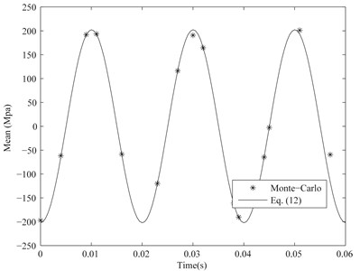
Fig. 5Standard deviation of the maximal fixed-end stress of the considered cantilever beam when CV= 0.005 and other parameters are the same as Section 2.1
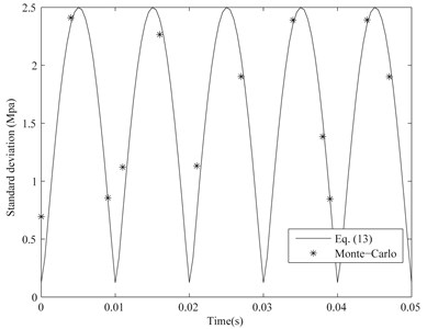
Fig. 6Correlation coefficient between maximal fixed-end stress and its time derivative of the considered cantilever beam when CV= 0.005 and other parameters are the same as Section 2.1
Then, the partial derivative of the expected number of crossings with respect to is:
where:
Then, the expected cumulative damage of the beam with normal distribution parameters and subjected to cyclic load during the time interval t1 to t2 could be calculated by substituting Eq. (25) and (26) into Eq. (20) and using the numerical integration method.
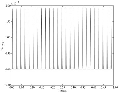
Using the proposed method, the expected instantaneous damages () of the cantilever beam with normal distribution parameters are shown in Fig. 7 and 8 when 0.005 and 0.010 respectively. Other parameters of the considered beam are the same as Section 2.1. The expected instantaneous damage of the discussed random cantilever beam subjected to cyclic load is the periodic function of the time and its amplitude with 0.010 is more than one with 0.005 from Fig. 7 and 8. The expected cumulative damage with 0.005 and 0.010 during one second are 4.945×10⁻⁴ and 1.742×10⁻³ and their corresponding lives (numbers of cycles to failure) are 1.072×10⁵ and 3.043×10⁴ respectively.
Fig. 7Expected instantaneous damage of the cantilever beam with normal distribution parameters and subjected to cyclic load when CV= 0.005 and other parameters are the same as Section 2.1
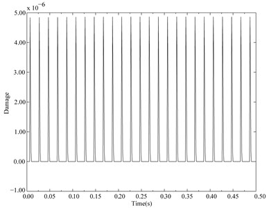
Fig. 8Expected instantaneous damage of the cantilever beam with normal distribution parameters and subjected to cyclic load when CV= 0.01 and other parameters are the same as Section 2.1
4. Conclusions
One method for estimating the life of the beam with normal distribution parameters and subjected to cyclic load was presented in this work. The random generalized displacement and velocity of the beam with random parameters at any time are the normal distributions when CVs of all random parameters are small (generally 0.01). Their means and variances could be accurately estimated by the random perturbation method. By compared with Monte-Carlo simulation, the means, variances and their correlation coefficient of the random dynamic stress and its time derivative could be estimated using the first-order approximation method in a Taylor series. The presented method could estimate the life of the beam with normal distribution parameters and subjected to cyclic load where the random dynamic stress is non-stationary and follows the normal distribution with the nonzero mean at any time .
References
-
Ge J., Sun Y., Zhou S. Fatigue life estimation under multiaxial random loading by means of the equivalent Lemaitre stress and multiaxial S-N curve methods. International Journal of Fatigue, Vol. 79, 2015, p. 65-74.
-
Larsena C., Irvineb T. A review of spectral methods for variable amplitude fatigue prediction and new results. Procedia Engineering, Vol. 101, 2015, p. 243-250.
-
Mrsnik M., Slavic J., Boltezar M. Frequency-domain methods for a vibration-fatigue-life estimation – application to real data. International Journal of Fatigue, Vol. 47, 2013, p. 8-17.
-
Braccesi C., Cianetti F., Lori G., Pioli D. Random multiaxial fatigue: a comparative analysis among selected frequency and time domain fatigue evaluation methods. International Journal of Fatigue, Vol. 74, 2015, p. 107-118.
-
Vidic G., Nagode M. Critical evaluation of frequency-domain approach for fatigue damage estimation. Journal of Engineering Materials and Technology, Vol. 136, Issue 3, 2014, p. 1-7.
-
Benasciutti D., Tovo R. Spectral methods for lifetime prediction under wide-band stationary random processes. International Journal of Fatigue, Vol. 27, 2005, p. 867-877.
-
He G., Chen H., He X. Fatigue behavior and influence factor analysis of the structure subject to multiaxial random loading. Journal of Vibroengineering, Vol. 17, Issue 7, 2015, p. 3620-3634.
-
Thakkar R. Exact Sinusoidal Simulation of Fatigue under Gaussian Narrow Band Random Loading. Retrospective Theses and Dissertations, Iowa State University, 1972
-
Eldogan Y., Cigeroglu E. Vibration fatigue analysis of a cantilever beam using different fatigue theories. Topics in Modal Analysis, Proceedings of the 31st IMAC, A Conference on Structural Dynamics, Conference Proceedings of the Society for Experimental Mechanics Series 45, Springer Verlag, Berlin, Vol. 7, 2013, p. 471-478.
-
Paulus M., Dasgupta A., Habtour E. Life estimation model of a cantilevered beam subjected to complex random vibration. Fatigue and Fracture of Engineering Materials and Structures, Vol. 35, Issue 11, 2012, p. 1058-1070.
-
Paulus M., Dasgupta A. Semi-empirical life model of a cantilevered beam subject to random vibration. International Journal of Fatigue, Vol. 45, 2012, p. 82-90.
-
Lin R., Huang P., Zhao C., Guo X., Zheng X. Prediction of fatigue lives of RC beams strengthened with CFL under random loading. Acta Mechanica Solida Sinica, Vol. 21, Issue 4, 2008, p. 359-363.
-
Lin R. The Methods for Predicting Fatigue Lives of RC Beams Strengthened with CFL Under Random Loads. Dissertation for Master’s degree, South China University of Technology, Guangzhou, 2005.
-
Wang X., Sun J. Random fatigue of a higher order sandwich beam with parameter uncertainties. Journal of Sound and Vibration, Vol. 260, Issue 2, 2003, p. 349-356.
-
Chen P., Soroka W. Impulse response of a dynamic system with statistical properties. Journal of Sound and Vibration, Vol. 31, Issue 3, 1973, p. 309-314.
-
Chen S. Vibration Theory of Structures with Random Parameters. Jilin Science and Technology Press, Changchun, 1990.
-
Gere J., Goodno B. Mechanics of Materials (8 Edition). CENGAGE Learning Custom Publishing, Boston, 2013.
-
Zhang Y., He X., Liu Q., Wen B. Robust reliability design of banjo flange with arbitrary distribution parameters. Journal of Pressure Vessel Technology – Transactions of the ASME, Vol. 27, Issue 4, 2005, p. 408-413.
-
Roberts J. Structural fatigue under non-stationary random loading. Proceedings of the Institution of Mechanical Engineers, Part C, Journal of Mechanical Engineering Science, Vol. 8, Issue 4, 1966, p. 392-405.
-
Rice S. Mathematical analysis of random noise. Bell System Technical Journal, Vol. 23, Issue 3, 1945, p. 282-332.
About this article
The work is supported by National Natural Science Foundation of China (Grant No. 51575095), Fundamental Research Funds for the Central Universities of China (Grant No. N140304006), China Ministry of Education New Century Excellent Person Support Plan (Grant No. NCET-12-0105) and Major State Basic Research Development Program of China (973 Program) (Grant No. 2014CB046303).
Li Changyou offers the idea and the most of the theoretical innovation of this article. The random dynamical response was analyzed and the most of the revision works of the manuscript were done by Wang Xuchu. The random dynamical stress was analyzed by Wang Wei. The prominent assistance in the theory analysis was offered by Zhang Yimin. The simulation of Section 3 was done by Guo Song.
