Wave displacement of rigid bodies and particles

Ragulskis, Kazimieras; Ragulskis, Liutauras

Journal of Vibroengineering

Browse Journal

Submit article

Published: 30 June 2013

Check for updates

Wave displacement of rigid bodies and particles

Kazimieras Ragulskis¹

Liutauras Ragulskis²

¹Kaunas University of Technology, Kaunas, Lithuania

²Vytautas Magnus University, Kaunas, Lithuania

Cite the article Download PDF

Downloads 1181

Abstract

The displacement of various particles and mechanical systems by waves finds wide use in technical devices, technological processes, takes place in non living and living nature. Here the system displaced by waves with four degrees of freedom is analyzed when one member of the system, while contacting with the working profile of the input member performing wave motion, provides motion to the output system.The obtained differential equations of motion of the system have been analyzed analytically and numerically. For the analytical investigation modification of the asymptotic method is used, which is based on the division of motion into the slow and quick motions. This method is justified when the frequencies of variation of slow motions are much smaller than the frequencies of quick motions.When the working surface of the input member moves according to the harmonic Rayleigh waves more detailed full investigations have been performed. The characteristics of transition to steady state and of stationary regimes of motions have been obtained, such as the conditions of existence and stability of the stationary regimes, curves of bifurcation, existing complicated motions.

1. Introduction

The conveyance of particles and bodies by propagating waves is an important scientific and engineering problem with numerous applications. Manipulation of bioparticles and gene expression profiling using travelling wave dielectrophoresis [1-3], segregation of particles in suspensions subject to alternative current electric fields [4], transport of sand particles and oil spills in coastal waters [5, 6], powder transport by piezoelectrically excited ultrasonic waves [7, 8] are just few examples of problems involving interaction between propagating waves and transported objects.

There is a large variety of waves of various types according to their shapes and laws of propagation [9-13]. This paper is focused on the displacement of systems with lumped parameters by one-dimensional periodic waves. This is important in a number of mechanical engineering applications. For the case of Rayleigh harmonic waves the investigations are performed in more detail.

2. The model of the system

The model of the system is presented in Fig. 1.

2.1. Kinematics

The coordinates of the moving points in the frame $X O Y$ read:

1

A_{1} (u, ξ), A_{2} (u, v), B_{1} (u + u_{1}, v + v_{1}), B_{2} (u - R s i n φ, v - R c o s φ),

where:

2

u = x + η, v = ξ, R = A_{1} B_{2} = A_{2} B_{2} .

The working profile of the input member 1 is given by:

3

η (x, t), ξ (x, t),

and the components of velocities of their contact point $A_{1}$ are:

4

{η^{'}}_{t}, {ξ^{'}}_{t} .

Fig. 1The model of the system: 1 – the working profile of the input member, 2 – contact member of the output system, 3 – member 1 may move according to two orthogonal directions with respect to member 2, 4 – a pendulum is attached to the member 2 by a hinge

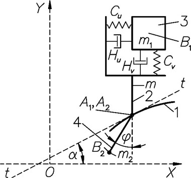
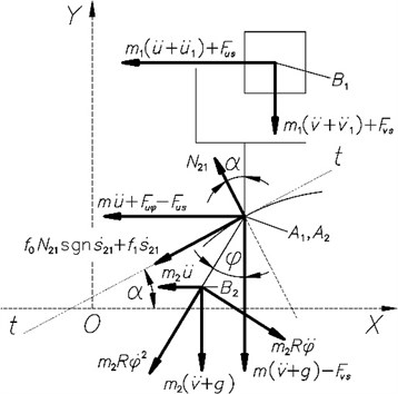
Fig. 2Forces acting in the system

The components of velocities and accelerations of contact point $A_{2}$ of member 2 read:

5

\dot{u} = (1 + {η^{'}}_{x}) \dot{x} + {η^{'}}_{t}, \dot{v} = {ξ^{'}}_{x} \dot{x} + {ξ^{'}}_{t},

6

\ddot{u} = (1 + {η^{'}}_{x}) \ddot{x} + {η^{″}}_{x x} {\dot{x}}^{2} + 2 {η^{″}}_{x t} \dot{x} + {η^{″}}_{t t}, \ddot{v} = {ξ^{'}}_{x} \ddot{x} + {ξ^{″}}_{x x} {\dot{x}}^{2} + 2 {ξ^{″}}_{x t} \dot{x} + {ξ^{″}}_{t t} .

Further the following relationships are met:

7

F_{1} = (1 + {η^{'}}_{x}) \ddot{u} + {ξ^{'}}_{x} \ddot{v} = a_{1} \ddot{x} + a_{2} {\dot{x}}^{2} + 2 a_{3} \dot{x} + a_{4},

F_{2} = - {ξ^{'}}_{x} \ddot{u} + (1 + {η^{'}}_{x}) \ddot{v} = b_{2} {\dot{x}}^{2} + 2 b_{3} \dot{x} + b_{4},

where:

8

a_{1} = {(1 + {η^{'}}_{x})}^{2} + {ξ^{'}}_{x}^{2}, a_{2} = (1 + {η^{'}}_{x}) {η^{″}}_{x x} + {ξ^{'}}_{x} {ξ^{″}}_{x x},

a_{3} = (1 + {η^{'}}_{x}) {η^{″}}_{x t} + {ξ^{'}}_{x} {ξ^{″}}_{x t}, a_{4} = (1 + {η^{'}}_{x}) {η^{″}}_{t t} + {ξ^{'}}_{x} {ξ^{″}}_{t t},

b_{2} = (1 + {η^{'}}_{x}) {ξ^{″}}_{x x} - {ξ^{'}}_{x} {η^{″}}_{x x}, b_{3} = (1 + {η^{'}}_{x}) {ξ^{″}}_{x t} - {ξ^{'}}_{x} {η^{″}}_{x t},

b_{4} = (1 + {η^{'}}_{x}) {ξ^{″}}_{t t} - {ξ^{'}}_{x} {η^{″}}_{t t} .

The angle $α$ of the tangent at the point of the profile $A_{1}$ with the axis $O X$ :

9

t a n α = \frac{{ξ^{'}}_{x}}{1 + {η^{'}}_{x}} .

The velocity of slippage of point $A_{2}$ with respect to point $A_{1}$ in the tangential direction takes the form:

${\dot{s}}_{21} = (\dot{v} - {ξ^{'}}_{t}) s i n α + (\dot{u} - {η^{'}}_{t}) c o s α,$

or:

10

{\dot{s}}_{21} = \sqrt{a_{1}} \dot{x} .

2.2. Differential equations of motion

The equations of dynamic equilibrium of the member 2 (Fig. 2) are:

11

(m + m_{2}) \ddot{u} + m_{2} R P_{u} - F_{u} + f_{1} {\dot{s}}_{21} c o s α = - N (s i n α + f_{0} s g n {\dot{s}}_{21} c o s α),

(m + m_{2}) (\ddot{v} + g) + m_{2} R P_{v} - F_{v} + f_{1} {\dot{s}}_{21} s i n α = N (c o s α - f_{0} s g n {\dot{s}}_{21} s i n α),

where $N$ is the normal force acting to the member 2 at the points $A_{1}$ and $A_{2}$ , $f_{0}$ and $f_{1}$ are the coefficients of dry and viscous friction:

12

P_{u} = - \ddot{φ} c o s φ + {\dot{φ}}^{2} s i n φ, P_{v} = \ddot{φ} s i n φ + {\dot{φ}}^{2} c o s φ,

F_{u} = H_{u} {\dot{u}}_{1} + C_{u} u_{1}, F_{v} = H_{v} {\dot{v}}_{1} + C_{v} v_{1},

and $g$ is the acceleration of gravity of the Earth.

Rearrangement of the equations (11) and taking into account the equations (2)-(9) yields:

13

(1 + {η^{'}}_{x}) I_{u} + {ξ^{'}}_{x} I_{v} + [- {ξ^{'}}_{x} I_{u} + (1 + {η^{'}}_{x}) I_{v}] f_{0} s g n {\dot{s}}_{21} + h α_{1} \dot{x} = 0,

14

R \ddot{φ} - \ddot{u} c o s φ + \ddot{v} s i n φ + g s i n φ + \frac{K_{φ}}{m_{2} R} \dot{φ} = 0,

15

\ddot{u} + {\ddot{u}}_{1} + F_{u} = 0,

16

\ddot{v} + {\ddot{v}}_{1} + F_{v} = 0,

where:

17

I_{u} = \ddot{u} + μ_{2} R P_{u} - μ_{1} \frac{F_{u}}{m_{1}}, I_{v} = \ddot{v} + g + μ_{2} R P_{v} - μ_{1} \frac{F_{v}}{m_{1}},

μ_{1} = \frac{m_{1}}{m + m_{2}}, μ_{2} = \frac{m_{2}}{m + m_{2}}, h = \frac{f_{1}}{m + m_{1}}, \dot{} = \frac{d}{d t},

$K_{φ}$ is coefficient of viscous friction.

3. Systems excited by traveling waves

In this case the equations (3) take the form:

18

η = η (ω t - k x), ξ = ξ (ω t - k x),

where $η$ and $ξ$ are periodic functions of their arguments.

The following notations are introduced:

19

ψ = ω t - k x, τ = ω t, β = k x, β_{1} = k u_{1}, β_{2} = k v_{1},' = \frac{d}{d τ} .

In this case equations (5)-(10) by taking into account the equations (18), (19) take the following form:

20

k u^{'} = 1 - c_{4} ψ^{'}, k v^{'} = c_{5} ψ^{'}, k u^{″} = - c_{4} ψ^{″} + c_{6} {ψ^{'}}^{2}, k v^{″} = c_{5} ψ^{″} + c_{7} {ψ^{'}}^{2},

k F_{1} = - c_{1} ψ^{″} + c_{2} {ψ^{'}}^{2}, k F_{2} = c_{3} {ψ^{'}}^{2},

where:

21

c_{1} = {(1 - k η^{'})}^{2} + k^{2} {ξ^{'}}^{2}, c_{2} = (1 - k η^{'}) k η^{″} - k^{2} ξ^{'} ξ^{″}, c_{3} = (1 - k η^{'}) k ξ^{″} + k^{2} ξ^{'} η^{″},

c_{4} = 1 - k η^{'}, c_{5} = k ξ^{'}, c_{6} = k η^{″}, c_{7} = k ξ^{″}, r = k R .

Differential equations of motion (13)-(17) by taking into account equations (18)-(21) read:

22

- c_{1} ψ^{″} + c_{2} {ψ^{'}}^{2} + c_{4} (μ_{2} r p_{u} - μ_{1} f_{u}) - c_{5} (\frac{k g}{ω^{2}} + μ_{2} r p_{v} - μ_{1} f_{v}) + [- c_{3} {ψ^{'}}^{2} + c_{5} (μ_{2} r p_{u} - μ_{1} f_{u}) + c_{4} (\frac{k g}{ω^{2}} + μ_{2} r p_{v} - μ_{1} f_{v})] f_{0} s g n {\dot{s}}_{21} + c_{1} \frac{h}{ω} (1 - ψ^{'}) = 0,

23

r φ^{″} + (c_{4} ψ^{″} - c_{6} {ψ^{'}}^{2}) c o s φ + (c_{5} ψ^{″} + c_{7} {ψ^{'}}^{2}) s i n φ + \frac{h_{φ}}{ω} φ^{'} + \frac{k g}{ω^{2}} s i n φ = 0,

24

- c_{4} ψ^{″} + c_{6} {ψ^{'}}^{2} + {β^{″}}_{1} + f_{u} = 0,

25

c_{5} ψ^{″} + c_{7} {ψ^{'}}^{2} + {β^{″}}_{2} + f_{v} = 0,

where:

26

p_{u} = - φ^{″} c o s φ + {φ^{'}}^{2} s i n φ, p_{v} = φ^{″} s i n φ + {φ^{'}}^{2} c o s φ,

f_{u} = \frac{h_{u}}{ω} {β^{'}}_{1} + {(\frac{n_{u}}{ω})}^{2} β_{1}, f_{v} = \frac{h_{v}}{ω} {β^{'}}_{2} + {(\frac{n_{v}}{ω})}^{2} β_{2},

h = \frac{f_{1}}{m + m_{2}}, h_{u} = \frac{H_{u}}{m_{2}}, h_{v} = \frac{H_{v}}{m_{2}}, n_{u}^{2} = \frac{C_{u}}{m_{2}}, n_{v}^{2} = \frac{C_{v}}{m_{2}}, h_{φ} = \frac{k K_{φ}}{m_{2} R} .

3.1. Case: harmonic traveling waves:

Following equalities are obtained according to (21) and taking into account (27):

27

η = A c o s (ω t - k x), ξ = B s i n (ω t - k x) .

28

c_{1} = {(1 + a s i n ψ)}^{2} + b^{2} {c o s}^{2} ψ, c_{2} = - (1 + a s i n ψ) a c o s ψ + b^{2} s i n ψ c o s ψ,

c_{3} = - (1 + a s i n ψ) b s i n ψ - a b s i n ψ c o s ψ,

c_{4} = 1 + a s i n ψ, c_{5} = b c o s ψ, c_{6} = - a c o s ψ, c_{7} = - b s i n ψ, a = k A, b = k B .

3.2. Analytical investigation for the case of slow motions when the average velocity of the output system is much smaller than the velocity of traveling waves

In this case the steady state motions and the transient ones which are near to them are sought in the following form:

29

ψ = ψ_{0} + \tilde{ψ}, φ = φ_{0} + \tilde{φ}, ψ_{0} = \bar{ψ^{'}} τ + \bar{ψ}, φ_{0} = \bar{φ^{'}} τ + \bar{φ},

where $\bar{ψ^{'}}$ and $\bar{φ^{'}} = \frac{m}{n} \bar{ψ^{'}}$ are average velocities in the steady state regimes:

30

m, n = 0, \pm 1, \pm 2, \dots, \frac{m}{n} \leq 1,

$\bar{ψ}$ and $\bar{φ}$ are slowly varying quantities, $\tilde{ψ}$ and $\tilde{φ}$ are quickly varying quantities.

For the determination of quick motions linear differential equations with constant coefficients are obtained. The latter are obtained from the main equations (22)-(26) by assuming in them that the dash over separate members denotes averaging with respect to time and the wave over the members means that their average values with respect to the period of time are equal to zero. Nonlinear autonomous differential equations are obtained for the determination of slow motions by assuming in the initial equations (22)-(26) $ψ$ and $φ$ according to the equations (30) and performing linearization over one time period.

Differential equations describing quick motions are obtained from equations (22)-(25) when $f_{0} = 0$ by taking into account the equations (30):

31

{\bar{c}}_{1} ({\tilde{ψ}}^{″} + \frac{h}{ω} \tilde{ψ^{'}}) = {\bar{ψ^{'}}}^{2} c_{2} (ψ_{0}) + μ_{1} r \tilde{({\bar{φ^{'}}}^{2} c_{4} (ψ_{0}) s i n φ_{0})} - {\bar{c}}_{4} μ_{1} f_{u}

- \tilde{(c_{5} (ψ_{0}) (\frac{k g}{ω^{2}} + μ_{2} r {\bar{φ^{'}}}^{2} c o s φ_{0}))} + \tilde{c_{1} (ψ_{0})} \frac{h}{ω} = 0,

32

r \tilde{φ^{″}} + \frac{k_{φ}}{ω} \tilde{φ^{'}} - {\bar{ψ^{'}}}^{2} c_{6} (ψ_{0}) c o s φ_{0} + {\bar{φ^{'}}}^{2} \tilde{(c_{7} (ψ_{0}) s i n φ_{0})} + \frac{k g}{ω^{2}} s i n φ_{0} = 0,

33

- {\bar{c}}_{4} \tilde{ψ^{″}} + {\bar{ψ^{'}}}^{2} c_{6} (ψ_{0}) + {β^{″}}_{1} + f_{u} = 0,

34

{\bar{ψ^{'}}}^{2} c_{7} (ψ_{0}) + {β^{″}}_{2} + f_{v} = 0,

where the upper dash means averaging with respect to the period, $f_{u}$ and $f_{v}$ are determined according to the equations (26), $c_{i}$ ( $i =$ 1, …,7) are determined according to the equations (28), (29).

The differential equations of slow motion respectively are only for the determination of $\bar{ψ}$ and $\bar{φ}$ , namely:

35

{\bar{c}}_{1} (\bar{ψ^{″}} + \frac{h}{ω} \bar{ψ^{'}}) = {\bar{ψ^{'}}}^{2} \bar{c_{2} (ψ_{0} + \tilde{ψ})} + μ_{1} r {\bar{φ^{'}}}^{2} \bar{c_{4} (ψ_{0} + \tilde{ψ}) \sin (φ_{0} + \tilde{φ})} - μ_{1} \bar{c_{4} (ψ_{0} + \tilde{ψ}) f_{u}}

- \frac{k g}{ω^{2}} \bar{c_{5} (ψ_{0} + \tilde{ψ})} - μ_{2} r {\bar{φ^{'}}}^{2} \bar{c_{5} (ψ_{0} + \tilde{ψ}) \cos (φ_{0} + \tilde{φ})} + \frac{h}{ω} \bar{c_{1} (ψ_{0} + \tilde{ψ})} = 0,

36

r \bar{φ^{″}} + \frac{k_{φ}}{ω} \bar{φ^{'}} - {\bar{ψ^{'}}}^{2} \bar{c_{6} (ψ_{0} + \tilde{ψ}) c o s (φ_{0} + \tilde{φ})} + {\bar{φ^{'}}}^{2} \bar{c_{1} (ψ_{0} + \tilde{ψ}) s i n (φ_{0} + \tilde{φ})}

+ \frac{k g}{ω^{2}} \bar{s i n (φ_{0} + \tilde{φ})} = 0 .

Further systems are analyzed starting from the simplest ones.

3.3. Case 1: system with one degree of freedom

First the problem is analyzed when the particle moves with a velocity much smaller than the velocity of the wave, that is $δ - 1 = ε \geq 0,$ $ε$ is a small quantity.

In this case the differential equations of the slow and quick motions are obtained on the basis of the equations (31) and (35) by taking into account the equations (28):

37

[1 + 0.5 (a^{2} + b^{2})] (\tilde{ψ^{″}} + \frac{h}{ω} \tilde{ψ^{'}}) = {\bar{ψ^{'}}}^{2} [- a c o s ψ_{0} - 0.5 (a^{2} - b^{2}) s i n 2 ψ_{0}]

- \frac{k g}{ω^{2}} b c o s ψ_{0} + \frac{h}{ω} [2 a s i n ψ_{0} - 0.5 (a^{2} - b^{2}) c o s 2 ψ_{0}] = 0,

38

[1 + 0.5 (a^{2} + b^{2})] (\bar{ψ^{″}} + \frac{h}{ω} \bar{ψ^{'}}) = - {\bar{ψ^{'}}}^{2} [a \bar{\cos (ψ_{0} + \tilde{ψ})} + 0.5 (a^{2} - b^{2}) \bar{s i n 2 (ψ_{0} + \tilde{ψ})}] + \frac{k g}{ω^{2}} b \bar{\cos (ψ_{0} + \tilde{ψ})}

+ \frac{h}{ω} [1 - 0.5 (a^{2} - b^{2}) + 2 a \bar{\sin (ψ_{0} + \tilde{ψ})} - 0.5 (a^{2} - b^{2}) \bar{c o s 2 (ψ_{0} + \tilde{ψ})}] = 0 .

Steady state regimes of quick motion according to the equation (37) are of the following type: $\tilde{ψ} = R_{1} c o s ψ_{0} + S_{1} s i n ψ_{0} + R_{2} c o s 2 ψ_{0} + S_{2} s i n 2 ψ_{0},$

and by substituting it into the equation (38), before this performing the expansion of it into a power series with respect to $\tilde{ψ}$ and taking into account only the linear part and after averaging it is obtained:

39

δ = 1 - \frac{a^{2}}{2 d_{1} S} [\frac{{(- δ^{2} + \frac{k g}{ω^{2}} d_{2})}^{2} + 4 {(\frac{h}{ω})}^{2}}{δ^{2} + {(\frac{h}{ω})}^{2}} + \frac{0.25 a^{2} {(1 - d_{2}^{2})}^{2} (δ^{4} + {(\frac{h}{ω})}^{2})}{4 δ^{2} + {(\frac{h}{ω})}^{2}}],

where:

40

d_{1} = 1 + 0.5 (a^{2} + b^{2}), d_{2} = \frac{b}{a} .

It is clear that:

41

δ = 1 - ε,

where $ε$ is a small quantity, on the right side of the equation (39) it is possible to assume $ε = 0$ and:

42

{δ |}_{δ = 1} = 1 - \frac{a^{2}}{2 d_{1}} [\frac{{(- 1 + \frac{k g}{ω^{2}} d_{2})}^{2} + 4 {(\frac{h}{ω})}^{2}}{1 + {(\frac{h}{ω})}^{2}} + \frac{0.25 a^{2} {(1 - d_{2}^{2})}^{2} (1 + {(\frac{h}{ω})}^{2})}{4 + {(\frac{h}{ω})}^{2}}] .

In the case when the particle moves with a velocity of the excited wave, it is:

43

δ = 0 .

In this case:

44

ψ = 0 \cdot τ + \bar{ψ} .

The differential equation of slow motion according to the equation (32) is the following one:

45

d_{1} (\bar{ψ^{″}} + \frac{h}{ω} \bar{ψ^{'}}) = a \{- \frac{k g}{ω^{2}} d_{2} c o s \bar{ψ} + \frac{h}{ω} [d_{1} + 2 s i n \bar{ψ} - 0.5 a (1 - d_{2}^{2}) c o s 2 \bar{ψ}]\} = Ψ (\bar{ψ}) .

Stationary values of $\bar{ψ}$ are found from the following equation:

46

Ψ (\bar{ψ}) = 0 .

Stable values of $\bar{ψ}$ are those which satisfy the following inequality:

47

\frac{\partial Ψ (\bar{ψ})}{\partial \bar{ψ}} = a \{\frac{k g}{ω^{2}} d_{2} s i n \bar{ψ} + \frac{h}{ω} [2 c o s \bar{ψ} + a (1 - d_{2}^{2}) s i n 2 \bar{ψ}]\} < 0,

and in case of the opposite sign of the inequality (47) there are unstable values.

The equation (47) may have four or two or none real solutions with respect to $\bar{ψ}$ . This means that the motions with the velocity of the wave exist or do not exist. When the motions with the velocity of the wave exist, which of them are stable and which are unstable is determined according to the roots of the characteristic equation.

The characteristic equation at the stationary points according to the equation (45) is the following one:

48

d_{1} λ^{2} + d_{1} \frac{h}{ω} λ - (\frac{\partial Ψ}{\partial \bar{ψ}}) = 0,

where:

49

\frac{\partial Ψ}{\partial \bar{ψ}} = a \{\frac{k g}{ω^{2}} s i n \bar{ψ} + \frac{h}{ω} [2 c o s \bar{ψ} + a (1 - d_{2}^{2}) s i n 2 \bar{ψ}]\} .

Roots of the equation (49) are:

50

λ_{1; 2} = - \frac{1}{2} \frac{h}{ω} \pm \sqrt{\frac{1}{4} {(\frac{h}{ω})}^{2} + d_{1}^{2} (\frac{\partial Ψ}{\partial \bar{ψ}})} .

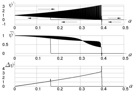
Unstable points $\bar{ψ}$ separate stable regimes, among them including stable regimes taking place at the velocity of the wave and at the velocity smaller than the velocity of the wave. Curves going through the unstable points are bifurcation curves.

Because in the stationary points of $\bar{ψ}$ , which are determined by the equation (46), may be four, two or zero real values, then also ${(λ_{1,2})}_{j}$ may be $j =$ 1, …,4, $j =$ 1, 2, $j =$ 0 $.$

Solving equation (45) with initial conditions from the infinitely small vicinity of the unstable point of $\bar{ψ}$ , which is determined by the equations (46) and (47), bifurcation lines are obtained.

Because stationary regimes may exist:

51

\bar{ψ^{'}} = δ and \bar{ψ^{'}} = 0,

so for the global representation the phase plane is used:

52

ψ^{'} = ψ^{'} (ψ^{″}) .

From the unstable points, which are determined by the equations (46) and (47), by integrating the differential equation (22), in which $p_{u} = p_{v} = f_{u} = f_{v} = f_{0} = 0$ and $c_{1}, c_{2}, c_{5}$ are determined by the equations (28), bifurcation curves are obtained.

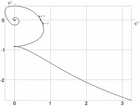
When $b = 1.5 a, \frac{h}{ω} = 0.5, \frac{k g}{ω} = 2$ slowly changing $a = a (ε τ)$ graphical relationships have been obtained $ψ^{'} = ψ^{'} (a),$ $\bar{ψ^{'}} = \bar{ψ^{'}} (a),$ ${ψ^{'}}_{max} - {ψ^{'}}_{min} = Δ ψ^{'},$ $ψ^{'} = ψ^{'} (ψ^{″}),$ (Fig. 3, 4) which reflect the dynamical qualities of the system.

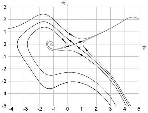
Fig. 3Transition to the steady state process when a= 0.25,hω= 0.5,kgω= 2 from the unstable point ψ-= 1.08825,Ψ'ψ-= 0.748257 (Fig. 3(a)) and from the stable point ψ-= 4.5421,Ψ'ψ-= –0.794566 (Fig. 3(b)), phase trajectories of motion and attractors (Fig. 3(c))

Transition to the steady state process when a= 0.25,hω= 0.5,kgω= 2 from the unstable point ψ-= 1.08825,Ψ'ψ-= 0.748257 (Fig. 3(a)) and from the stable point ψ-= 4.5421,Ψ'ψ-= –0.794566 (Fig. 3(b)), phase trajectories of motion and attractors (Fig. 3(c))

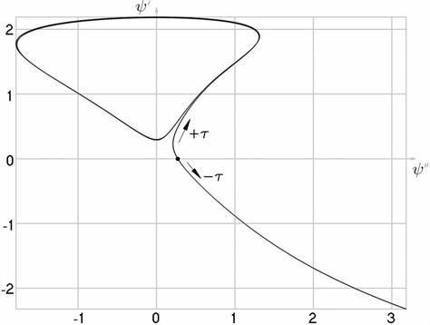
a)

b)

c)

Fig. 4Steady state motions of the system

3.4. Case 2: system with two degrees of freedom according to the coordinates $ψ$ and $φ$

In this case in the equations of motion (22) and (23) it is assumed $f_{u} = f_{v} = f_{0} = 0 .$

Here the motions are investigated, for which:

53

\bar{ψ^{'}} = \bar{φ^{'}} = δ .

By taking into account the equations (27) and (28), the quick and slow equations (22) and (23) become the following ones:

54

d_{1} (ψ^{″} + \frac{h}{ω} ψ^{'}) = r_{0} + r_{1} c o s ψ_{0} + s_{1} s i n ψ_{0} + s_{1 φ} s i n φ_{0} + r_{2} c o s 2 ψ_{0}

+ s_{2} s i n 2 ψ_{0} + r_{2 ψ φ} c o s (ψ_{0} + φ_{0}),

55

φ^{″} + \frac{h_{φ}}{ω} φ^{'} = r_{0}^{*} + s_{1 φ}^{*} s i n φ_{0} + r_{2 φ}^{*} \cos (ψ_{0} + φ_{0}),

where it is denoted:

56

r_{0} = [1 + 0.5 (ω^{2} + b^{2})] \frac{h}{ω}, r_{1} = - (a + \frac{k g}{ω^{2}} b), s_{1} = 2 \frac{h}{ω} a, s_{1 φ} = μ_{2} r δ^{2},

r_{2} = - 0.5 (a^{2} - b^{2}) \frac{h}{ω}, s_{2} = - 0.5 (a^{2} - b^{2}) δ^{2}, r_{2 ψ φ} = - μ_{1} r δ^{2},

r_{0}^{*} = - 0.5 (a^{2} - b^{2}) δ^{2} \cos (\bar{ψ} - \bar{φ}), s_{1 φ}^{*} = - \frac{h_{φ} g}{ω^{2}}, r_{2 φ}^{*} = 0.5 (a - b) δ .

From the equations (54) and (55) the quick motions are:

57

\tilde{ψ} = R_{1} c o s ψ_{0} + S_{1} s i n ψ_{0} + R_{1 φ} c o s φ_{0} + S_{1 φ} s i n φ_{0} + R_{2} c o s 2 ψ_{0} + S_{2} s i n 2 ψ_{0}

+ R_{2 ψ φ} \cos (ψ_{0} + φ_{0}) + S_{2 ψ φ} \sin (ψ_{0} + φ_{0}),

58

\tilde{φ} = R_{1 φ}^{*} c o s φ_{0} + S_{1 φ}^{*} s i n φ_{0} + R_{2 φ}^{*} \cos (ψ_{0} + φ_{0}) + S_{2 φ}^{*} \sin (ψ_{0} + φ_{0}),

and the slow motions are:

59

d_{1} (\bar{ψ^{″}} + \frac{h}{ω} \bar{ψ^{'}}) = r_{0} - r_{1} \bar{\tilde{ψ} s i n ψ_{0}} + s_{1} \bar{\tilde{ψ} c o s ψ_{0}} + s_{1 φ} \bar{\tilde{φ} c o s φ_{0}}

- 2 r_{2} \bar{\tilde{ψ} s i n 2 ψ_{0}} + 2 s_{2} \bar{\tilde{ψ} c o s 2 ψ_{0}} - 2 r_{2 ψ φ} \bar{(\tilde{ψ} + \tilde{φ}) s i n (2 δ τ + \bar{ψ} + \bar{φ})},

60

r \bar{φ^{″}} + \frac{h_{φ}}{ω} \bar{φ^{'}} = r_{0}^{*} + s_{1 φ}^{*} \bar{\tilde{φ} c o s φ_{0}} - r_{2 φ}^{*} \bar{(\tilde{ψ} + \tilde{φ}) s i n (2 δ + \bar{ψ} + \bar{φ})} .

By taking into account the equations (57) and (58), the equations (59) and (60) become the following ones:

61

d_{1} (\bar{ψ^{″}} + \frac{h}{ω} \bar{ψ^{'}}) = r_{0} - 0.5 r_{1} S_{1} + 0.5 s_{1} R_{1} + 0.5 s_{1 φ} R_{1 φ}^{*}

+ r_{2} [- S_{2} - R_{2 ψ φ} \sin (\bar{ψ} - \bar{φ}) - S_{2 ψ φ} \cos (\bar{ψ} - \bar{φ})]

+ s_{2} [R_{2} + R_{2 ψ φ} \cos (\bar{ψ} - \bar{φ}) - S_{2 ψ φ} \sin (\bar{ψ} - \bar{φ})]

+ r_{2 ψ φ} [R_{2} \sin (\bar{ψ} - \bar{φ}) + S_{2} \cos (\bar{ψ} - \bar{φ}) - S_{2 ψ φ} - S_{2 φ}^{*}],

62

r \bar{φ^{″}} + \frac{h_{φ}}{ω} \bar{φ^{'}} = s_{0}^{*} + 0.5 s_{1 φ}^{*} R_{1 φ}^{*} + r_{2 φ}^{*} [R_{2} \sin (\bar{ψ} - \bar{φ}) - S_{2} \cos (\bar{ψ} - \bar{φ}) - S_{2 ψ φ} - S_{2 φ}^{*}],

or:

63

d_{1} (\bar{ψ^{″}} + \frac{h}{ω} \bar{ψ^{'}}) = A_{1} \cos (\bar{ψ} - \bar{φ}) + A_{2} \sin (\bar{ψ} - \bar{φ}) + A_{3},

r \bar{φ^{″}} + \frac{h_{φ}}{ω} \bar{φ^{'}} = A_{1}^{*} \cos (\bar{ψ} - \bar{φ}) + A_{2}^{*} \sin (\bar{ψ} - \bar{φ}) + A_{3}^{*},

or by taking into account the equation (59) it is obtained:

64

d_{1} \frac{h}{ω} δ = A_{1} \cos (\bar{ψ} - \bar{φ}) + A_{2} \sin (\bar{ψ} - \bar{φ}) + A_{3} = 0,

\frac{h_{φ}}{ω} δ = A_{1}^{*} \cos (\bar{ψ} - \bar{φ}) + A_{2}^{*} \sin (\bar{ψ} - \bar{φ}) + A_{3}^{*} = 0 .

From the equations (64) $δ$ and $(\bar{ψ} - \bar{φ})$ are found. On the right side by assuming $δ = 1$ in the coefficients $A_{j}, A_{j}^{*}$ it is obtained:

65

(\frac{h}{h_{φ}} A_{1}^{*} - A_{1}) \cos (\bar{ψ} - \bar{φ}) + (\frac{h}{h_{φ}} A_{2}^{*} - A_{2}) \sin (\bar{ψ} - \bar{φ}) + \frac{h}{h_{φ}} A_{3}^{*} - A_{3} = 0 .

From the equation $(\bar{ψ} - \bar{φ})$ is found. One of them can be freely assigned any value, because the system of differential equations is autonomous.

Further investigation is performed in the same way as in case 1. The only difference here is in the fact that four stationary regimes at $0 < δ < 1$ can not exist. In this case only two stationary regimes exist, one of them is stable and one of them is unstable. Also even one stable and one unstable regime may not exist.

When the output system moves at the velocity of the exciting wave, then the obtained results are of the same type as for the case 1.

4. Conclusions

The main objective of this paper is to analyze transverse and longitudinal deformations of the working profile of the input member which displaces the output member, consisting from rigid members according to one coordinate. More detailed analysis is performed when the working profile of the input member is moving according to traveling harmonic Rayleigh waves, and one member of the output system has point contact with the profile of the input member.

Approximate analytical modified asymptotic method is used for the investigation of the stationary motions of the output system, which is based on the division of motion into the slow and quick motions. The characteristics of motion have been obtained, which are valid for the regimes when the output system moves at a much lower average velocity than the velocity of the exciting wave.

Bifurcations and complicated motions and control of the system have been determined by using analytical and numerical methods.

References

Chou C. F., Tegenfeldt J. O., Bakajin O., Chan S. S., Cox E. C., Darnton N., Duke T., Austin R. H. Electrodeless dielectrophoresis of single- and double-stranded DNA. Biophys. J., Vol. 83, 2002, p. 2170-2179.

Search CrossRef
Cui L., Korgan H. Design and fabrication of travelling wave dielectrophoresis structures. J. Micromech. Microeng., Vol. 10, 2000, p. 72-79.

Search CrossRef
Talary M. S., Burt J. P. H., Tame J. A., Pethig R. Electromanipulation and separation of cells using travelling electric fields. J. Phys. D Appl. Phys., Vol. 29, 1996, p. 2198-2203.

Search CrossRef
Dusiaud A. D., Khusid B., Acrivos B. A. Particle segregation in suspensions subject to high gradient ac electric fields. J. Appl. Phys., Vol. 88, 2000, p. 5463-5473.

Search CrossRef
Wael N. H., Ribberink J. S. Transport processes of uniform and mixed sands in oscillatory sheet flow. Coastal Eng., Vol. 52, No. 9, 2005, p. 745-770.

Search CrossRef
Wang S. D., Shen Y. M., Zheng Y. H. Two-dimensional numerical simulation for transport and fate of oil spills in seas. Ocean Eng., Vol. 32, 2005, p. 1556-1571.

Search CrossRef
Mracek M., Wallaschek J. A system for powder transport based on piezoelectrically excited ultrasonic progressive waves. Mater. Chem. Phys., Vol. 90, No. 2-3, 2005, p. 378-380.

Search CrossRef
Ragulskis M., Sanjuan M. A. F. Transport of particles by surface waves: a modification of the classical bouncer model. New Journal of Physics, Vol. 10, 2008, article no. 083017.

Search CrossRef
Ragulskis K. M. Mechanisms on a Vibrating Basis (Dynamics and Stability). Kaunas, Institute of the Lithuanian Academy of Sciences, 1963, 232 p., (in Russian).

Search CrossRef
Ganiev R. F., Ukrainsky L. E. Non-Linear Wave Mechanics & Technologies. Moscow: R&C Dynamics, 2008, 712 p.

Search CrossRef
Nonlinear Problems of Theory of Vibrations and Control Theory. Vibration Mechanics. For the 80-th Anniversary from the Birth of I. I. Blekhman. Edited by Beleckiy V. V. and others, St. Petersburg, Nauka, 2009, 528 p., (in Russian).

Search CrossRef
Ragulskis K., Spruogis B., Ragulskis M. Transformation of Rotational Motion by Inertia Couplings. Vilnius, Technika, 1999, 236 p.

Search CrossRef
Ragulskis M., Sakyte E. An explicit equation for the dynamics of a particle conveyed by a propagating wave. Mathematical and Computer Modeling of Dynamical Systems, Vol. 15, No. 4, 2009, p. 395-405.

Search CrossRef

About this article

Received

02 April 2013

Accepted

03 June 2013

Published

30 June 2013

Keywords

traveling waves

transient motions

stationary state

stability

bifurcation

This is an open access article distributed under the Creative Commons Attribution License, which permits unrestricted use, distribution, and reproduction in any medium, provided the original work is properly cited.