Finding Chebyshev series periodic solutions of nonlinear vibration systems via optimization method

1. Introduction

Chebyshev polynomials are one of the most important basis functions in numerical approximation [1, 2]. A Chebyshev series expansion can give precise approximations while reducing the Runge phenomenon [3]. It has been proved that a 15 to 18 terms shifted Chebyshev series of the first kind can accurately approach the trigonometric function [4] as well as the Floquet transition matrix (FTM) of high-dimension systems in stability analysis [5]. Although the use of Chebyshev series for solving ordinary differential equations has begun early [6], only recently it was applied to the study of periodic systems [5, 7-13]. In addition to reducing order of nonlinear periodic systems [12, 13] and solving delay-differential equations [14, 15], shifted Chebyshev series have been used to solve the response of nonlinear vibration systems [16, 17].

The nonlinear vibration system is widespread in mechanical, civil, aviation and other engineering fields. Since the periodic solution represents system steady state motion, the periodic solution and its stability are of important research value. Although the research for solving nonlinear vibration system has made great progress [18-22], there is still lack of general methods for solving an arbitrary nonlinear vibration system. Improving application scope, enhancing solution accuracy and reducing computational complexity of the solving method should be explored further [23]. While in the periodic-solution stability analysis, existing methods for calculating approximate FTM are generally cumbersome and of low-precision [24], or even worse may draw wrong conclusions on certain problems [25].

In order to obtain more precise analytical solutions and overcome the shortcomings in stability analysis, a method for solving Chebyshev series periodic solutions of nonlinear vibration systems is suggested. In the method the periodic solutions are expanded in the form of Chebyshev series with unknown coefficients. Then solving of the unknown coefficients is transformed to a nonlinear optimization issue on calculating the minimum residual force over a prime cycle. Compared with the current methods, the attractive feature of this method is as follows. Firstly, the high-accuracy analytical periodic solutions of nonlinear vibration systems can be obtained. The assumption of small parameters is abandoned and the high-dimension nonlinear vibration system is also applicable. Secondly, the initial value of optimization method can be reasonably estimated without trying blindly, which will effectively adjust solving precision. Thirdly, when periodic solutions are expanded in the form of shifted Chebyshev series of the first kind, the FTM can be obtained rapidly and accurately by integral operation without the help of the special methods for solving approximate FTM, and it will be beneficial to the stability analysis of periodic solutions.

The remaining paper is organized as follows. Section 2 gives the properties of the shifted Chebyshev series of the first kind. Section 3 outlines the method for solving the Chebyshev series periodic solution of nonlinear vibration systems. Two examples, namely Duffing equation and helicopter rotor coupling motion equations, are given to demonstrate the accuracy and validity of the suggested method in Section 4. Finally, the paper ends with conclusions in Section 5.

2. Properties of the shifted Chebyshev series of the first kind

Chebyshev polynomials of the first kind are defined as follows:

and are orthogonal over the interval $[-1,1]$ about the weight function $w\left(t\right)={(1-t^2)}^{-1/2}$.

For ease of use, take the change of variable $t^{*}=(t+1)/2$, then shifted Chebyshev polynomials of the first kind are obtained over the interval $[0,1]$, and they satisfy the following relationship:

According to the properties of shifted Chebyshev polynomials of the first kind, any function which is continuous in the interval $[0,\mathrm{}1]$ can be expanded into the shifted Chebyshev series of the first kind [4] as:

where $a_r$ are Chebyshev coefficients, and they can be obtained from:

The integral of Chebyshev polynomials satisfies:

and $\left[G\right]$ is the integral operator matrix.$\left\{T^{*}\right(t\left)\right\}$ is a column vector of the polynomials, defined as:

where ${\left\{\right\}}^T$ denotes the transpose operation of the quantity $\left\{\right\}$.

The product of Chebyshev polynomials satisfies:

and $\left[Q\right]$ is the integral operator matrix.

The other related theories of shifted Chebyshev series, the value of operator matrix $\left[G\right]$ and $\left[Q\right]$ are given in references [4, 5, 16, 17].

3. The method of analysis

Consider the following strongly nonlinear vibration system:

where $X\left(t\right)={\left\{x_1\right(t)x_2\left(t\right)\dots x_n(t\left)\right\}}^T$ is an $n\times 1$ column vector and $f\left(X\right(t),t)$ is a function of period $T$.

In nonlinear dynamics, compared with the determination of equilibrium points, the existence of periodic motions and the number of periodic solutions are even more difficult to ascertain. In general we only solve a part of periodic motions of the nonlinear vibration system. Let $X\left(t\right)={\{x_1\left(t\right)x_2\left(t\right)\dots x_n(t\left)\right\}}^T$ denote a periodic solution of Eq. (9) such that the periodic solution can be expressed as $m$ terms shifted Chebyshev series:

where $T_i^{*}$ is the $i$th shifted Chebyshev polynomial of the first kind, $p_{ij}$ and $q_{ij}$ are unknown Chebyshev coefficients. In order to estimate optimization initial value reasonably, the periodic solution should be expanded in harmonic series (or other series) at the same time:

where $a_{ik}$ and $b_{ik}$ are $(2N+1)\cdot n$ unknown harmonic series coefficients. For a single-period orbit $j=1$, for a period-doubling orbit $j=2^n$ and $n$ is the number of period-doubling bifurcation. Taking periodic solution of single-periodic orbit for example, we expand every harmonic of Eq. (12) in terms of the shifted Chebyshev series of the first kind, i.e.:

where $T_i^{*}$ is the $i$th shifted Chebyshev polynomial of the first kind, $\omega =2\pi /T$ and each column of matrix $\left[c_{ij}\right]$ is from the $m$ terms Chebyshev coefficients of the corresponding trigonometric function.

Since the domain of shifted Chebyshev series of the first kind is $[0,\mathrm{}1]$, the transformation $t=T\cdot s$$(s\in [\mathrm{0,1}\left]\right)$ must be done in order to normalize the period to 1. In actual calculation it is only necessary to expand the nonlinear vibration system equation into shifted Chebyshev series of the first kind and to replace $\omega$ with $2\pi$, $t$ with $s$, $T_i^{*}\left(t\right)$ with $T_i^{*}\left(s\right)$. Transpose the right side of Eq. (9), then in symbolic form residual force $R\left(s\right)$ can be written as:

where ${\left[\stackrel{-}{T}\right(s\left)\right]}_{n\times nm}^T=I\otimes {[T_0^{*}\left(s\right)T_1^{*}\left(s\right)T_2^{*}\left(s\right)\dots T_{m-1}^{*}(s\left)\right]}^T$, $\otimes$ represents matrix Kronecker product. $\left[I\right]$ is the identity matrix. $\left[F\right(a_{ik},b_{ik}\left)\right]$ is an $nm\times 1$ column vector. Obviously, in the case of exact solutions, residual $R$ equals to $0$ on arbitrary time point in a primary cycle. Let $R_i\left(s\right)$ be the row component of residual force $R\left(s\right)$. The total error between the exact solutions and periodic solutions, see Eq. (10), is equivalent to the sum of the absolute value of all time points in a cycle. It can be expressed as an unconstrained nonlinear optimization problem, i.e.:

The unknown coefficients $a_{ik}$ and $b_{ik}$ can be obtained via local optimization algorithm such as quasi-Newton method [26]. Since initial value selection will affect optimization results of local optimization algorithm, the number of harmonic terms in Eq. (13) can be adjusted in order to limit optimization initial value in a reasonable range. For simplicity we can directly reference to the harmonic terms of harmonic balance method (HBM). Then according to Eq. (13), Eq. (14) and Eq. (16) the unknown Chebyshev coefficients $p_{ij}$ and $q_{ij}$ can be calculated. Note that the periodic solution of engineering models usually has a clear physical meaning (such as in Section 4.2.2) and a closed interval of the feasible region can be estimated. Then the interval optimization algorithm can be used to seek global optimal solutions, while it will greatly increase the time complexity and computational complexity, and sometimes it is not necessary.

When the periodic solution is expressed in the form of shifted Chebyshev series, the periodic solution stability can be analyzed as follows. Suppose that a perturbation $\Delta x\left(t\right)$ is imposed to the known periodic solution $x_0\left(t\right)$, i.e.:

Substitute Eq. (17) into the system equation and omit the higher order small amount. Then a linearized system with respect to $\Delta x\left(t\right)$ can be obtained:

By linear periodic system theory and Chebyshev series operation properties, we only need to integrate the linearization system Eq. (18) over the interval $[0,\mathrm{}1]$ with each column of the identity matrix as the integral initial value separately. Then the linearization-system state vector at the end point of the period is the corresponding column vector of FTM $\Phi \left(T\right)$ [4]. According to Floquet theory, if the eigenvalue norms of FTM are less than 1, the periodic solution of the system is asymptotically stable, otherwise it is unstable.

The shifted Chebyshev polynomial of the first kind, multiplication and integral operator matrix used in calculating residual force, objective function and FTM are given in references [4, 5, 16, 17]. In this paper a 15 terms shifted Chebyshev series of the first kind is adopted.

4. Examples

4.1. Application to the Duffing system

Consider the Duffing system with cubic nonlinearities:

19

$\ddot{x}+ax+b\dot{x}+c{x}^3=d\mathrm{c}\mathrm{o}\mathrm{s}\left(\omega t\right),$

where $a=4$, $b=2$, $c=17$, $d=5$, $\omega =2$. When solving the shifted Chebyshev series periodic solution with the suggested method, we must normalize the period to 1 by transforming the time variable $t$ to $2\pi s/\omega$$\left(s\in \left[\mathrm{0,1}\right]\right)$. Then we expand Eq. (19) into shifted Chebyshev series, and calculate the system residual $R$ via multiplication and integral operator matrix. Finally quasi-Newton method can be used to seek optimal solutions of objective function. Table 1 shows the unknown coefficients of periodic solution obtained by the optimization method (3-term harmonic) and HBM (7-term harmonic).

Table 1Coefficients of approximate analytical periodic solution

Coefficient	Optimization method	Coefficient	HBM
$p_0$	0.000214327013	$a_0$	0
$p_1$	0.55117695	$a_1$	0.550665369
$p_2$	0.37818696117	$b_1$	0.37846670826
$p_3$	0.00059928746	$a_2$	0
$p_4$	-0.0009649196	$b_2$	0
$p_5$	0.0157754674	$a_3$	0.0162381788
$p_6$	0.051302781	$b_3$	0.0515055873
$p_7$	0.00044608728	$a_4$	0
$p_8$	0.00055906966	$b_4$	0
$p_9$	-0.0022438111	$a_5$	-0.00222665
$p_{10}$	0.0023410744	$b_5$	0.003084981
$p_{11}$	-0.0000682019	$a_6$	0
$p_{12}$	0.00056548798	$b_6$	0
$p_{13}$	-0.0002677232	$a_7$	-0.0002695199
$p_{14}$	-0.000180024115	$b_7$	0.000017709946

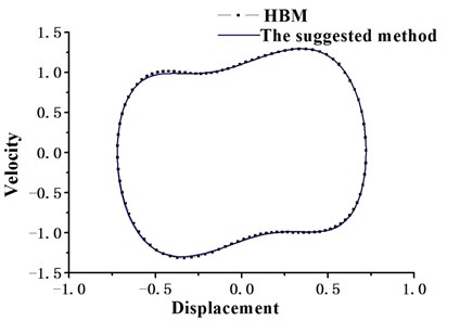
Fig. 1 and Fig. 2 show the residual curves obtained by the two methods over one time cycle. It can be seen that even the number of harmonic terms adopted in the suggested method is fewer than that of HBM, the periodic solution obtained still has greater accuracy than HBM. The reason is that in the suggested method adjusting the harmonic expansion terms is equivalent to changing the optimization initial value reasonably, and the objective function aims to reduce the error between the supposed periodic solution and the exact solution. Obviously the suggested method is apt to get a higher accuracy periodic solution. The phase portraits of Duffing system obtained by optimization method and HBM are displayed in Fig. 3, and both of them coincide very well. The optimization method not only requires expanding fewer harmonic items than HBM (i.e. solving fewer unknown coefficients), but also reduces the residual from 10^-3 to 10^-7 order of magnitude.

Fig. 1The residual curve of HBM

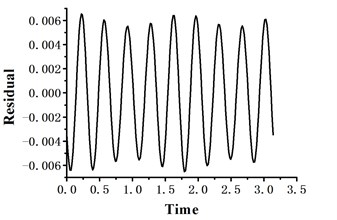
Fig. 2The residual curve of the suggested method

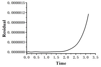
Fig. 3The phase portrait of Duffing system

According to the linear periodic system theory and the Chebyshev series operation property, take each column of identity matrix as the integral initial condition respectively. The state vector obtained at the end of the cycle via integration is the corresponding column of FTM. One of the norms of the eigenvalue (Floquet multiplier) of FTM is 10.91, which is greater than 1. Then the periodic solution of Duffing equation is unstable.

4.2. Helicopter rotor system

Rotor response and its stability is an important research topic in helicopter dynamics. Rotor dynamics model is a time-varying differential equation group containing nonlinear structure, inertial and aerodynamic loads. It is usually calculated by HBM, time finite element method (TFEM) or numerical integration algorithm. Since numerical integration algorithm is sensitive to integration initial value, solving rotor response usually adopts HBM or TFEM.

4.2.1. Application to the articulated rotor system

Take the articulated helicopter rotor motion for example. Consider flapping/lagging coupled movements in rotating plane, as shown in Fig. 4 and Fig. 5. Suppose that each blade has the same properties. The flapping/lagging coupled equations are established as follows:

20

$\left\{\begin{array}{l}{\int }_e^R{\eta }_{\beta }(r-e)mdr\ddot{\beta }+{\int }_e^R{\eta }_{\beta }rmdr\beta {\Omega }^2+K_{\beta }\left(\beta -{\beta }_p\right)={\int }_e^R\left(r-e\right)F_{z}dr,\\ {\int }_e^R(r-e){\eta }_{\xi }mdr\ddot{\xi }+{\int }_e^{R}e{\eta }_{\xi }mdr\xi {\Omega }^2+{\int }_e^R{\eta }_{\beta }{\eta }_{\xi }mdr2\Omega \beta \dot{\beta }+K_{\xi }\xi ={\int }_e^R(r-e)F_{x}dr.\end{array}\right.$

Fig. 4The force diagram of articulated rotor blade flap movement

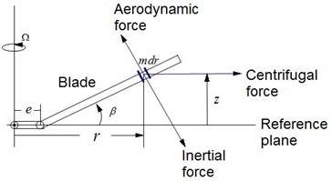
Fig. 5The force diagram of articulated rotor blade lag movement

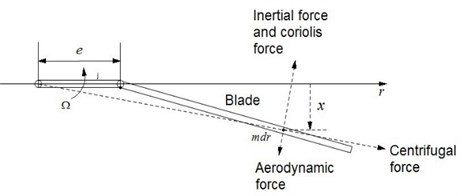
The symbols in the above equations have been described in references [27, 28]. $F_x$ is the aerodynamic force parallel to the disc plane. $F_z$ is the aerodynamic force vertical to the disc plane. Where:

21

$F_x=\frac{1}{2}\left(u_P{u}_T\theta -u_P^2\right)+\frac{C_d}{2a}{u}_T^2,$

22

$F_z=\frac{1}{2}\left(u_T^2\theta -u_P{u}_T\right),$

23

$u_T=r+\mu \mathrm{s}\mathrm{i}\mathrm{n}\left[\psi \right],$

24

$u_P=\lambda +r\dot{\beta }+\beta \mu \mathrm{c}\mathrm{o}\mathrm{s}\left[\psi \right].$

Table 2Main parameters of the articulated helicopter rotor system

Illustration	Unit	Value
Rotor radius	m	5.345
Rotor speed	rad/s	40.42
Rotor shaft anteversion angle	deg	2
Chord length	m	0.35
Blade number		3
Flapping hinge overhang amount	m	0.205
Blade twist angle	deg	-12
Airfoil lift line slope	rad-1	6.2
Airfoil zero lift incidence	deg	0.75
Rotor solidity		0.06253
Mass moment around flapping hinge	kg⋅m	88.68
Inertia moment around flapping hinge	kg⋅m2	306.01

Let us assume that advance ratio $\mu$ equals to 0.2 and take Drees inflow model. For ease of calculation, the parameters not listed in the Table are supposed equal to 0.

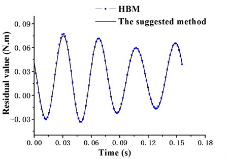
Transform the blade motion equations into state equations and take the periodic solution Eq. (13) into Eq. (20). Normalize the system period to 1. Then residual force $R_i$ of each motion equation can be obtained. When the periodic solutions are expanded as the 2-term harmonics, the variance averages of flapping and lagging motion equations obtained by HBM are 1.90047 and 0.073. Obviously, it is a wrong conclusion, because large magnitude harmonic terms of the periodic solution are omitted. Meanwhile, the system variance averages obtained by optimization method (quasi-Newton method) are 0.443 and 0.128, which can be considered comparatively accurate. The reason is that in the suggested method harmonic series is only used to correct the optimization initial value. The final result is the local optimal value in the vicinity of the initial value and the periodic solution is still approximated by a 15 terms shifted Chebyshev series. When expanded in the form of the 3-term harmonics, the total variance averages obtained by optimization method are 9.8 % lower than that of HBM in a cycle. Fig. 6 and Fig. 7 show the residual curves of the blade flapping/lagging motions when periodic solutions are expanded to the 3-term harmonics.

Fig. 6Residual curve of flapping movement (3-term harmonics)

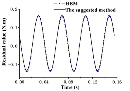
Fig. 7Residual curve of lagging movement (3-term harmonics)

Note that the objective function of this issue can also be solved by global optimization algorithm. As $\beta$ and $\xi$ on behalf of the flapping and lagging periodic solutions we can estimate a reasonable feasible region, i.e. a closed interval range according to actual situation. Then the periodic solutions can be converged to global optimal solutions by deterministic methods, while the calculation complexity will increase significantly and the time cost becomes unacceptable. It can be seen through the calculation results that by adjusting the optimization initial values local optimization method (quasi-Newton method) can also generate satisfying results. When we take the 7-term harmonic expansion, the system variance average can reach up to 10^-10 order of magnitude and the flapping and lagging movement phase portraits are shown in Fig. 8 and Fig. 9.

The periodic solution stability can be analyzed by Floquet theory. According to the linear periodic system theory and the Chebyshev series operation property we calculate the FTM. All the norms of eigenvalue of FTM are 0.0963 and 0.6802, less than 1. Therefore when advance ratio $\mu$ equals to 0.2, the helicopter rotor coupling motion is asymptotically stable.

Fig. 8Phase portrait of blade flapping movement

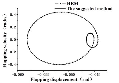
Fig. 9Phase portrait of blade lagging movement

4.2.2. Application to the hingeless rotor system

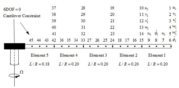
Consider the hingeless helicopter rotor system. Establish rotor blade motion equation in rotating coordinate via finite element method. The blade space finite element is shown in Fig. 10.

Fig. 10Blade space finite element

The blade motion equation using the symbolic representation is:

25

$\stackrel{-}{M}\ddot{q}+\stackrel{-}{C}\dot{q}+\stackrel{-}{K}q-\stackrel{-}{F}=0,$

where $q\left(t\right)=\{u_1,v_1,{v^{\text{'}}}_1,w_1,{w^{\text{'}}}_1,{\varphi }_1,\dots ,u_{14},{\varphi }_{10},u_{15}\}$ is the total node displacement vector on a single blade. $u$, $v$, $w$, $\varphi$ represent the stretching, lagging, flapping and twist elastic displacements for each node on the blade elastic axis. In this example the blade parameters are adopted as BO-105 rotor parameters in [29], where quasi-steady aerodynamic force and Drees inflow model are considered.

In order to reduce the computation time and equation dimension, we take the first six order intrinsic modes in calculation. Then Eq. (25) transforms into an equation with respect to mode coordinate $p\left(t\right)$:

26

$\dot{p}\left(t\right)=A\left(p\left(t\right),t\right)\cdot p\left(t\right)+C\left(t\right),$

where $p\left(t\right)={\{p_1,p_2,p_3,p_4,p_5,p_6,{\dot{p}}_1,{\dot{p}}_2,{\dot{p}}_3,{\dot{p}}_4,{\dot{p}}_5,{\dot{p}}_6\}}^T$ is dimensionless mode degree of freedom. A numerical method, named TFEM, is usually used to solve the response of high-dimension nonlinear rotor system model.

Fig. 11Dimensionless mode degree of freedom phase portraits on blade tip position

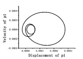
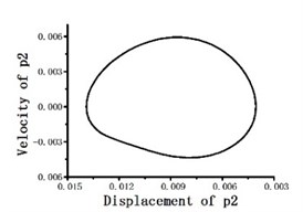
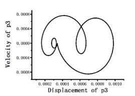
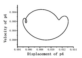
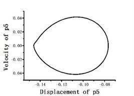
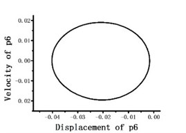
Fig. 12Blade tip flapping response phase portrait

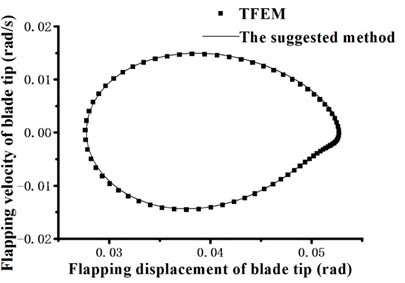
Fig. 13Blade tip lagging response phase portrait

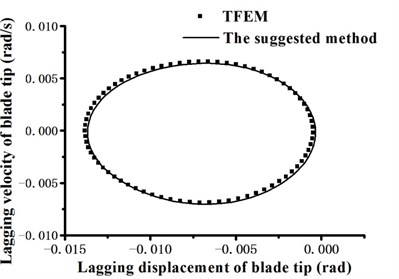
Fig. 14Blade tip twist response phase portrait

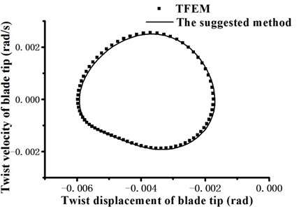
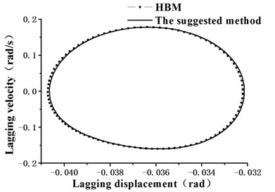
When periodic solution is expanded to 3-term harmonics as optimization initial value, the total variance averages obtained by optimization method reach up to 10^-6 order of magnitude, which is slightly more accurate than TFEM (take 15 time elements and 5-order shape function). The dimensionless mode degree of freedom phase portraits on blade tip position are shown in Fig. 11. Then we return the mode degree of freedom to physical degree of freedom. Fig. 12 to Fig. 14 show the flapping, lagging and twist response phase portraits. The periodic solutions obtained by optimization method coincide very well with the numerical results of TFEM. It proves that the suggested method is accurate and effective.

According to Floquet theory, all the norms of eigenvalues of FTM are less than 1. Therefore when advance ratio $\mu$ equals to 0.2, the periodic motion of this hingeless rotor is asymptotically stable.

5. Conclusions

In this paper, using the good properties of shifted Chebyshev series in numerical approximation field, proceeding from optimization of system residual force, the analytical periodic solution in the form of shifted Chebyshev series of the first kind is obtained. Compared with HBM, when the periodic solution is expanded in fewer or the same harmonic terms, the suggested method owns higher accuracy. When solving the high-dimension nonlinear system, it can still obtain a high precision analytical solution. In periodic solution stability analysis the FTM can be obtained directly and accurately by the integral operation of Chebyshev series without the help of special numerical approach for calculating approximate FTM. Examples show that in addition to solving low-dimensional system, this method also can be used to calculate the periodic solution and to analyze the stability of high-dimensional nonlinear vibration system, such as the helicopter rotor system. It indicates that finding Chebyshev series periodic solutions of nonlinear vibration systems via optimization method is accurate and effective.