A new transient field balancing method of a rotor system based on empirical mode decomposition

1. Introduction

Dynamic balancing is one of the key techniques in modern industry, it is an important measure to ensure the safe and stable operation, improve performance, and extend the service life of the equipment. Unbalance occurs when the principle axis of the moment of inertia does not coincide with the axis of the rotation. To eliminate the unbalance, various balancing techniques have been developed [1, 2]. The influence coefficient method is based on linear vibration theory, the linear relationship between the corrected value and measured value is utilized to calculate correction weights. Different from the influence coefficient method, Modal balancing realize the whole balancing by calculating a sets of correction weights and applied to eliminate each modal component gradually with the assumption that different modal component are orthogonal to each other. The present dynamic balancing techniques, including influence coefficient method and modal balancing method, mainly concentrate on the constant rotating speed case, obtaining the vibration responses of original unbalance or trial weights in steady-state conditions. In practical application, this not only reduces the efficiency of dynamic balancing, but also causes great harm to the equipment when balancing speed is close to the critical speed [3]. Meanwhile, it is difficult for a rotor to work steadily at the certain speed, especially for machines work with time varying load, such as wind turbine generators, etc. If we can use some proper method to process the accelerating response data under variable speed condition, the unbalance can be identified quickly, avoiding unnecessary damages to the rotor at the same time.

The run-up or run-down process of rotating machinery is important. The thermal, stress, and running state change gradually. During the procedure, machines cross all speeds from zero to rating speed and are subjected to oscillating forces of increasing or decreasing frequency [4]. Its vibration signals are non-stationary and manifest large amplitude fluctuation in time domain. These vibration signals of the procedure carry abundant dynamic information of the machine and can be useful for condition monitoring and fault diagnosis, especially the information not obtained from steady-state running vibration signals.

However, it is a challenge to develop and adopt effective signal processing techniques that can extract amplitude and phase information for dynamic balancing because of the non-stationary characteristic of the run-up vibration signals. The conventional fast Fourier transform (FFT) based signal processing techniques usually result in false information when deal with non-stationary signals, because these techniques are founded on the basis that the signals being analyzed are stationary and linear. Wavelet transform is a time-frequency analysis method and decomposes a signal into a set of wavelet coefficients levels with different resolution. It is difficult to develop a wavelet base function that correlates well with the characteristics of the practical signal [5]. Empirical mode decomposition (EMD) is an adaptive and unsupervised method. EMD decomposes a signal into a set of almost orthogonal intrinsic mode functions (IMFs) based on the local characteristic time scales in time domain. The overall and local characteristics can be obtained by analyzing these IMFs. Moreover, the base functions are determined by the signal itself. It makes EMD suitable for processing non-stationary signals and distinct from the traditional method. The applications of EMD include rainfall analysis [6] to rotor fault diagnosis [7].

This paper focuses on the IMFs derived from the EMD to extract the features of rotating frequency faults from the run-up vibration signals of large rotating machinery. The interference from environmental noise and some irrelevant components are removed. Moreover, this kind of IMFs is relatively easy to understand and especially useful for the analysis of non-stationary, non-linear time series and further realization of transient balancing method based on holobalancing technique.

2. Empirical mode decomposition

EMD method introduced by Huang et al. is an innovative time-series analysis tool in comparison with traditional methods such as Fourier methods, wavelet methods, and empirical orthogonal functions. A signal will be broken down into its component IMFs by the sifting process of EMD. The result is a set of very nearly orthogonal functions and the number of functions in the set depends on the original signal. A more detailed and comprehensive description can be found in [8, 9].

The vibration signals of mechanical equipment are usually composite signal because of the complexities of mechanical systems and the interference of background noise. EMD is developed to decompose such composite signal into a set of components called IMF, which is embedded in the signal and can be very useful for feature extraction and fault identification. (1) In the whole data set, the number of extrema and the number of zero-crossings must either equal or differ at most by one. (2) At any point, the mean value of the envelope defined by local maxima and the envelope defined by the local minima is zero. The EMD process of a signal $x\left(t\right)$ can be described as follows:

(1) Identify all the local extrema, and then interpolate the local maxima and the local minima by cubic spline line to form upper and lower envelops respectively.

(2) Designate the mean of upper and lower envelops as $m_1$, and the difference between the signal $x\left(t\right)$ and $m_1$ as $h_1$:

(3) Verify $h_1$ whether satisfy the definition of IMF, if not, treat $h_1$ as the original signal and repeat step (1), (2) until $h_1$ becomes an IMF, then define $c_1=h_1$, $c_1$ is the first IMF obtained from the original data.

(4) Subtract $c_1$ from the original signal $x\left(t\right)$ to obtain the first residue $r_1$:

Treat $r_1$ as the original signal and repeat the steps above until the residue $r_n$ becomes a monotonic function from which no more IMF can be extracted or satisfy the predefined decomposition stop criteria. At the end of the decomposition procedure we obtain a collection of IMFs $c_i\left(i=1,2,\dots ,n\right)$ and a residue $r_n$:

Thus, the original signal $x\left(t\right)$ is decomposed into $n$-empirical modes and a residue $r_n$. The IMFs $c_1,c_2,\dots ,c_n$ include different local characteristic time scale and different frequency bands ranging from high to low, while the residue $r_n$ represents the mean trend of $x\left(t\right)$.

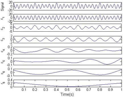
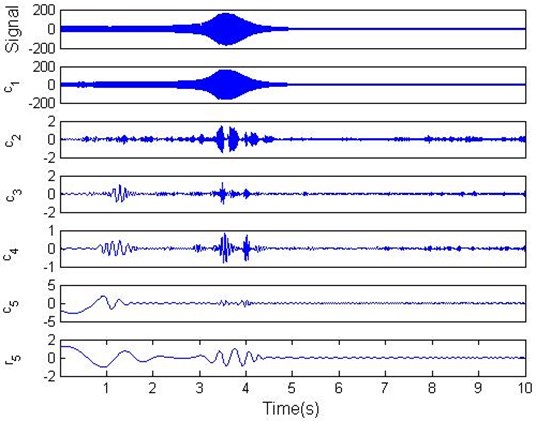
To demonstrate the process of EMD, investigate the following simulation signal:

The simulation signal is composed of two cosine waves with different frequency. The original signal and the decomposition result by EMD are shown in Fig. 1. It can be seen from Fig. 1 that the components $c_1,c_2,c_3$ respectively corresponding to the 30 Hz cosine waves, amplitude modulation cosine waves and 10Hz cosine waves, while $c_4,c_5,c_6$ are the illusive components of the decomposition. The illusive components are weak and often caused by the spline fitting error. Generally, EMD can identify and extract components with different local characteristic time scale from the original signal successfully.

Fig. 1IMFs and residual of the simulation signal

3. Holospectral technique

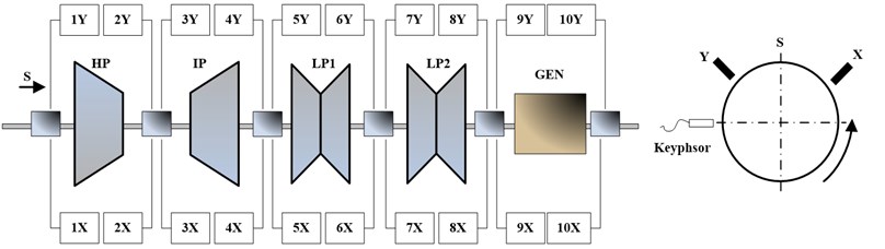
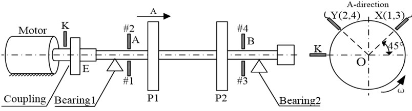
Fig. 2 shows the arrangement of sensors in a 300 mW turbo-generator unit. The rotor vibration can be obtained by two eddy current probes, which are presented by $iX,iY,i=1,...,10$ in Fig. 2, perpendicularly mounted across each bearing section. The high-pressure rotor, intermediate-pressure rotor, low-pressure rotor 1 and low-pressure rotor 2 of the turbine are indicated by the symbols HP, IP, LP1, LP2 separately, and the characters GEN present the generator of the turbine. This paper defines that the phase is the lag angle of key phasor pulse signal relative to the first forward zero of the vibration waveform.

The vibration components with rotating frequency in the $i$th measuring section, derived from two mutually perpendicular directions $X$ and $Y$, can be expressed as:

where $A_i$, $B_i$ are amplitudes, ${\alpha }_i$, ${\beta }_i$ are initial phases, $f$ is working frequency, $s_{xi}$ and $c_{xi}$ are the sine and cosine coefficients of the signal $x_i$, while $s_{yi}$ and $c_{yi}$ are the sine and cosine coefficients of the signal $y_i$. In general, the orbit constructed by the signals $x_i$ and $y_i$ is not a circle, but an ellipse. So the motion of a rotor is a complex spatial motion, which can not be objectively and reliably detected with just one single sensor. In most traditional balancing methods, only the vibration information in one measuring direction is used. It is based on the assumption of equal rigidity in different circumferential directions of rotor-bearing system. The analysis errors would occur when the rigidity is different.

Fig. 2The arrangement of sensors in a 300 MW turbine generator unit

From the viewpoint of information fusion, the holospectrum integrates the two vibration signals in a bearing section as a whole but not as individual measuring directions, which can fully reflect the vibration behavior of a rotor system. The initial phase point (IPP) is defined as the point on 1X ellipse (rotating frequency orbit), where the key slot on the rotor locates straightly opposite to the key-phasor. In this paper, the IPPs are used to analysis vibrations of a rotor system in balancing process, and may reduce errors and improve the balancing accuracy.

For the convenience of vector processing in balancing, the first harmonic frequency ellipse can be expressed as an array:

where $n$ is the number of measuring sections. The coordinates of IPPs in first frequency ellipses are $IP{P}_i=[c_{xi},c_{yi}]$.

The three-dimensional holospectrum integrates all first frequency ellipses, and therefore provide full vibration information of a rotor system as a whole simultaneously in all bearing sections, which can be expressed by the following matrix:

In this paper, the matrix of 3D-holospectrum is used to describe comprehensive vibration responses of a rotor system. Under the precondition of the linearity, it can simplify the computing of the vibration responses. For example, the initial unbalance responses are $\left\{\begin{array}{c}{x}_i=A_i\sin \left(2\pi ft+{\alpha }_i\right)\\ y_i=B_i\sin \left(2\pi ft+{\beta }_i\right)\end{array}\right.$ or $r_i=[s_{xi},c_{xi},s_{yi},c_{yi}]$, and added the trial weights, the vibration responses with trial weights are $\left\{\begin{array}{c}{\stackrel{-}{x}}_i={\stackrel{-}{A}}_{i}sin(2\pi ft+{\stackrel{-}{\alpha }}_i)\\ {\stackrel{-}{y}}_i={\stackrel{-}{B}}_{i}sin(2\pi ft+{\stackrel{-}{\beta }}_i)\end{array}\right.$ or $r_i=[{\stackrel{-}{s}}_{xj},{\stackrel{-}{c}}_{xj},{\stackrel{-}{s}}_{yj},{\stackrel{-}{c}}_{yj}]$, then the net response caused only by trial weights in the $i$th measuring section can be expressed as $\Delta r_i={\stackrel{-}{r}}_i-r_i$. For the vibration responses in all measuring sections, the matrix equation is:

4. Procedure of transient field balancing

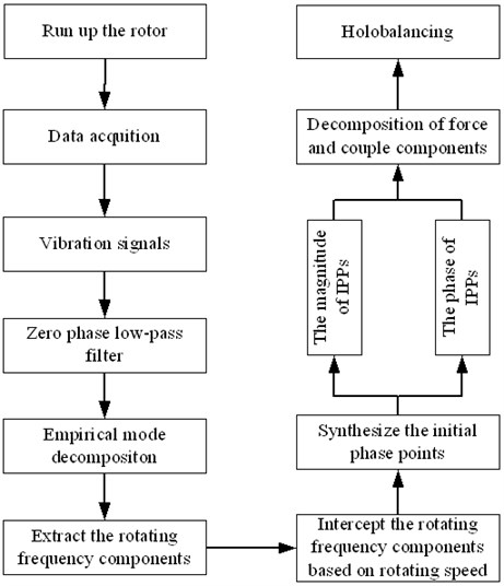
Given the amplitude and frequency modulation characteristic of the rotor run up vibration signals, it is difficult to adopt effective methods acquiring accurate amplitude and phase information of the unbalance responses. Compared with the traditional signal analysis method, EMD is somehow suit to processing the run up signals, since it’s an adaptive and data-driven method. Holobalancing is a development of the typical balancing methods and can improve the efficiency and precision of balance. The transient balancing method presented in this paper utilizes EMD to extract rotating frequency components from the run up vibration signals, and synthesizes the initial phase points of different rotating speeds with the aid of the key phase signal, and then the holobalancing method is adopted to realize the balance of the rotor system. The flowchart of the proposed method is shown in Fig. 3.

The key to implement efficient dynamic balancing is picking up precise amplitude and phase of the rotor’s unbalanced vibration [10]. Practically, the more data points can be sampled in one vibration period, the more accurate amplitude and phase can be obtained. Therefore, the implemented balancing will be more successful with higher probability. The presented transient balancing method extracts vibration information from run-up signals of the rotor system; consequently, the data points obtained in one vibration period are relatively scarce. To pick up amplitude and phase of unbalanced vibration signal accurately, the method first utilizes the zero phase low-pass filter to remove high frequency components, the aim is to eliminate the influence of those components and preserve the phase information at the same time. Secondly, as mentioned above, the holo-balancing technique takes the initial-phase point (IPP) as balancing target; the information needed to synthesize the IPP is obtained by intercepting the rotating frequency components based on rotating speed, which can be calculated from the key phase impulses. Compared with the traditional FFT method, this is a more direct way and can pick up more accurate amplitude information.

Fig. 3The flowchart of transient balancing method

4.1. Zero phase low-pass filter

Zero phase low-pass filters can reduce high frequency components of the original signal and therefore improve the efficiency and accuracy of EMD. Compared with the normal filter, it can eliminate the phase distortion and preserve the phase information of the original signal [11, 12]. Define the original signal sequence as $x\left(i\right),i=0,1,\dots ,n$, and the time domain reverse sequence as $y\left(i\right)=x\left(n-i\right),i=0,1,\dots ,n$. Extend $x\left(i\right)$ and $y\left(i\right)$ to the whole time axis, then given the bilateral $Z$-transformation:

9

$Y\left(z\right)=\sum _{n=-\infty }^{\infty }y\left(n\right)z^{-n}=\sum _{n=-\infty }^{\infty }x\left(-n\right)z^{-n}=\sum _{n=-\infty }^{\infty }x\left(n\right){\left(z^{-1}\right)}^{-n}=X\left(\frac{1}{z}\right).$

According to the relationship between the bilateral $Z$-transformation of the original signal sequence and the domain reverse sequence, a zero phase low-pass filter can be constructed as shown in Fig. 4, where $H\left(z\right)$ represents the transfer function of normal low-pass filter.

Fig. 4The flow chart of zero phase low-pass filter

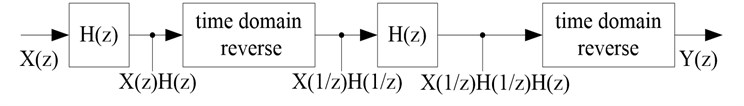
From Fig. 4, $Y\left(z\right)$ can be written as:

10

$Y\left(z\right)=X\left(z\right)H\left(z\right)H\left(\frac{1}{z}\right).$

Define $z=e^{jw}$ and substitute it into Equation (10), then Equation (10) becomes:

11

$Y\left(e^{jw}\right)=X\left(e^{jw}\right)H\left(e^{jw}\right)H\left(e^{-jw}\right)=X\left(e^{jw}\right){\left|H\left(e^{jw}\right)\right|}^2.$

As shown in Equation (11), the spectrum of output signal sequence is equal to the spectrum of input signal sequence multiplied by a real number. The amplitude of the original signal is changed due to the influence of filter transfer function, while the phase information is preserved. Therefore the phase distortion produced in filter process and baseline drift of low-frequency signal can be eliminated effectively. In this paper, the fifth order Butterworth filter is selected, considering Butterworth filter has the most smooth filter performance. Further more, since the maximum speed of the rotor kit system is 4000 rpm in the following experiment, the cut-off frequency of the zero phase low-pass filter is set as 70 Hz.

4.2. The extraction of rotating frequency component

In order to eliminate high frequency components, the original run-up vibration signals were processed by a zero phase low-pass filter, whose cut-off frequency is initialized larger than the highest rotating frequency of the run-up stage. EMD is a set of adaptive high-pass filters, the cut-off frequency and bandwidth of which change depend on the signal itself and decomposition process, then the decomposition results are arranged from high to low order of frequency. According to the above two major points, one can determine that the first IMF is the rotating frequency component. Fig. 5 shows the EMD decomposition results of a rotor run-up vibration signal, it can be noticed from Fig. 5 that the IMF $c_1$ is the rotating frequency component.

Fig. 5Rotating frequency component

5. Experiments and discussion

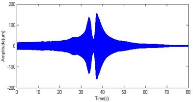
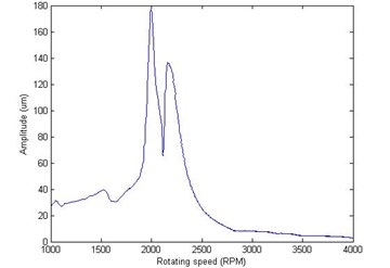
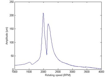
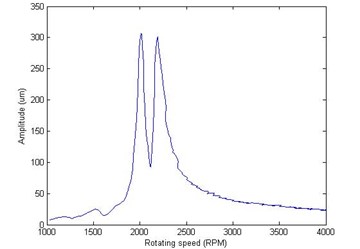
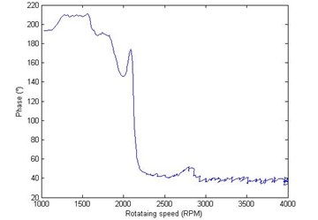
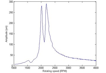
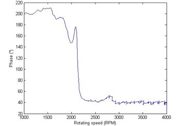
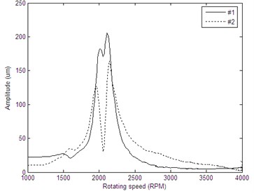
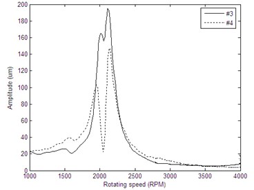
In this section, the proposed transient balancing method is verified on a test rig. The structure sketch of the test rig and the configuration of transducer are illustrated in Fig. 6, where transducers #1-#4 measure the vibration of the cross-section A and B, while the transducer #5 is key phase sensor and it collects key phase pulses to compute rotating speed of the rotor. In order to eliminate the disturbance of higher-order unbalance and concentrate on investigating the effect of the method to balance the first-order unbalance, the rotor system is balanced at 4000 rpm firstly. Set the sampling frequency as 2048 Hz, and the transient accelerating response of the rotor system is measured in the speed range of 0-4000 rpm. The waveform of bush #1 and #2 are shown in Fig. 7 and Fig. 8 respectively. As is shown in Fig. 7 and Fig. 8, the maximum vibration amplitude is more than 200 um at resonance, while the vibration amplitudes under other speeds are small, therefore it’s essential to correct the first order of unbalance.

Fig. 6The structure sketch of the test rig

Firstly, sampling the original run-up vibration signals and the corresponding key phase signal, utilize the zero phase low-pass filter to eliminate high frequency components of the original vibration signals, then extract rotating frequency components by EMD and acquire rotating speed of rotor system by computing the key phase signal. Intercept the rotating frequency components based on rotating speed and synthesize initial phase point according to the equation (13). The amplitude and phase information of initial phase point of the measuring plane A and B are shown in Fig. 9.

Fig. 7The vibration signal of bush #1

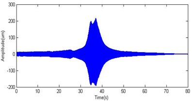
Fig. 8The vibration signal of bush #2

Next, after estimating the azimuth of unbalance mass according to the phase information of the original vibration signals, as well as the mechanical lag angle and the natural vibration characteristic at resonance, trial weights $T_A=$ 0.8 g∠90°, $T_B=$ 0.8 g∠90° were installed in the correction plane $P_1$ and $P_2$. Then start up the rotor system again and measure the vibration signals of the rotor with trials weights. According to the original vibration signals and trail weight vibration signals, the unbalance responses of both measuring plane A and B due to pure trial weight can be derived. Repeat the step 1 to acquire the initial phase point of pure trial weights. The amplitude and phase information of initial phase point due to pure trial weights are demonstrated in Fig. 10.

Since the main purpose is to balance the first-order unbalance and the phase information change remarkably nearby the critical speeds, the balance speed should be chosen as about 90 % of the first critical speed. The first critical speed of the rotor system is about 2100 rpm, therefore the balance speed is selected as 1900 rpm. Table 1 shows the detailed calculated data of the balance speed with the signal amplitude given in um and the phase angle given in degree.

Due to the restriction of the correction mass and angle of the correction plane, the actual correction masses added on plane A and B are both 0.6 g∠90°.

Fig. 9The initial phase point of original vibration signal: a) the amplitude of IPP in cross-section A, b) the phase of IPP in cross-section A, c) the amplitude of IPP in cross-section B, d) the phase of IPP in cross-section B

a)

b)

c)

d)

Fig. 10The initial phase point of vibration signals due to pure test weights: a) the amplitude of IPP in cross-section A, b) the phase of IPP in cross-section A, c) the amplitude of IPP in cross-section B, d) the phase of IPP in cross-section B

a)

b)

c)

d)

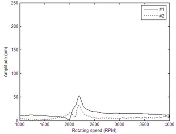
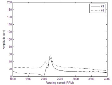
Measure the vibration of the rotor system after adding correction masses, the amplitudes of the vibration signals at resonance before and after balance can be seen in Table 2. As shown in Table 2, the amplitudes at the first critical speed have been reduced significantly after balancing. The vibration amplitudes of measuring plane A reduced from 206 um, 164.2 um to 52.47 um, 33.36 um respectively, while the amplitudes of measuring plane B reduced from 195.2 um, 147.1 um to 58.39 um, 50.5 um respectively. Meanwhile, the mean square vibration value also has been reduced significantly, range from 179.68 um before balancing to 49.56 um after balancing. The Hilbert envelop curves of original vibration signals and the balanced vibration signals are given in Fig. 11.

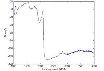
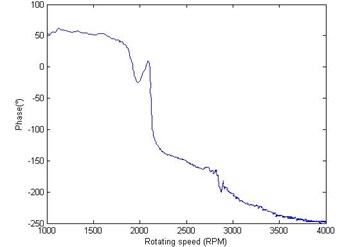
Fig. 11Bode diagrams of rotor run-up vibration signals: a) the rotating frequency bode diagram of cross-section A before balance, b) the rotating frequency bode diagram of cross-section B before balance, c) the rotating frequency bode diagram of cross-section A after balance, d) the rotating frequency bode diagram of cross-section B after balance

a)

b)

c)

d)

6. Conclusions

In this paper, a new transient balancing method based on non-stationary information is proposed in this paper. The empirical mode decomposition is described and applied to process the rotor run-up vibration signals, which are non-stationary and carry abundant dynamic information of the rotor system. The proposed method is applied to analyze and balance a rotor system with large vibration amplitude at the critical speed. The application results show that the proposed method is able to reduce the vibration amplitude significantly and achieve satisfactory balance effect.