Abstract
The calculation of response power spectrum of elastic thin plates, the common load-carrying structures in engineering, under distributed random load has been suffering from many problems, such as low efficiency and complicated computation which cause a lot of inconvenience for engineering applications. Therefore, a fast algorithm is introduced in this article to address above problems. Firstly, the function of the cross power spectrum function is projected onto orthogonal domain of multi-dimension Legendre polynomial, and the infinite distributing information is expressed by finite parameters. Secondly, the dynamic response computation of distributed random load is transformed into that of distributed harmonic load. Thirdly, the response power spectrum density for each frequency point can be obtained by vector multiplication. The fast algorithm is accurate; and its efficiency is much higher than a regular algorithm. Moreover, the fast algorithm conveniently illustrates the coherences of distributed random load. Finally, the fast algorithm is compared with a regular algorithm computation. The high efficiency and precision of the fast algorithm is demonstrated in this paper.
1. Introduction
Thin plate is a very common structure in engineering. Aircrafts and satellites, for instance, consist of many thin plates or stressed structures. In these circumstances, thin plates are mostly subjected to distributed dynamic load [1], especially distributed random load. Though it is relatively simple to calculate the direct problem under distributed determinate load, the calculation of structural dynamic response under distributed random load is quite complicated and inefficient [2, 3]. The calculation of structural dynamic response under distributed random load is usually simplified in engineering, which consequently magnifies the error [4-8]. In addition, the calculation of dynamic random response focuses on the structure due to multi-points excitation [9-13]. Few studies involve the calculation of structure random response due to the distributed random load. This paper proposes a new fast algorithm for the calculation of response power spectrum density of thin plates under distributed random load with the prerequisite of linear elasticity. The fast algorithm is an accurate and highly efficient method; and the above-mentioned difficulties in calculation of structural dynamic response under distributed random load can be satisfactorily resolved by means of the fast algorithm, so it may be useful for engineering problem involving response analysis of distributed random load.
There are mainly three methods to calculate structural response power spectrum density [14]: CQC (Complete Quadratic Combination) [15-18], SRSS (Square Root of the Sum of Squares) [19-21], and PEM (Pseudo-Excitation Method) [22, 23] proposed by Lin Jiahao. CQC is an accurate algorithm since it not only takes the square items of the main mode shapes, but also considers the coupling items. However, its efficiency is terrible. For elastic thin plates, the formula of CQC method is displayed as Eq. (1):
where and represent cross-spectrum density of response and cross-spectrum density of excitation between points and respectively. is mode shape of mode at point , is modal response frequency function of mode , and , represent the effect range of variants and , respectively. All the following symbols are treated same.
In order to reduce the calculation of CQC method, a simplified method which ignores all the coupling items in Eq. (1) is applied in engineering. It is called SRSS method. For elastic thin plates, the formula of SRSS method is shown as Eq. (2):
However, SRSS, when applied to structures with close vibration modes or large damping, suffers from large errors due to its assumption of independence among responses of all vibration modes.
PEM has been developed for mulit-input-multi-output stationary/non-stationary random vibration response problem since 1980s, thus it is a CQC algorithm with high efficiency and simple procedure [9-13]. Essentially, it approximates the random input in basic dynamic equation with a virtual determinate harmonic input and conducts vector multiplication for every single frequency to obtain response power spectrum density. Maily, this method is discussed for multiple inputs. A fast algorithm of PEM for one-dimensional continuous beam was developed [8], but the calculation of response power spectrum density of thin plates under distributed random load has not yet been involved.
The fast algorithm is proposed for accurate calculation of response power spectrum density of structures under line-distributed (one-dimensional) or plane-distributed (two-dimensional) random load on the thin plate. First, one-dimensional Legendre orthogonal polynomials are introduced to establish multi-dimensional ones. Second, the function of cross-power spectrum density, which is complicated to distribute on thin plate structures, is decomposed in orthogonal domain of multi-dimensional Legendre polynomials. Third, based on CQC method, the calculation of response power spectrum density of distributed random load is replaced with that of distributed determinate load; and by conducting vector multiplication for every single frequency, the response power spectrum density is thus gained. Regular approximated and the fast algorithms are programmed and evaluated in efficiency and precision to validate the advantages of the fast algorithm. The result of Nastran (the software for finite element analysis) demonstrates the correctness of the fast algorithm. Besides, the fast algorithm overcomes Nastran’s shortage that it can only compute the load model whose distributed load is completely coherent. In fact, not all distributed load is completely coherent, for example, fluctuating winds; if the stationary distributed random excitation is partial coherent, Nastran does not work. So, it is necessary to develop the fast algorithm which can calculate the structure random response under arbitrarily coherent distributed random load.
2. Theory
2.1. Multi-dimensional Legendre orthogonal polynomials
Located within a real span and with weighting function Legendre orthogonal polynomials [24, 25] can be described as follows:
In , recurrence formula of Legendre polynomials can be derived as below:
Based on the above one-dimensional Legendre orthogonal polynomials, two-dimensional orthogonal polynomials can be established as . According to the orthogonality of one-dimensional Legendre orthogonal polynomials, the orthogonality of two-dimensional ones is easily proved as follows:
It can also be proved that the established two-dimensional Legendre orthogonal polynomials possess the characteristics of parity and recurrence. As a result, constructs a series of two-dimensional orthogonal basis functions. Furthermore, multi-dimensional orthogonal polynomials can be constructed similarly as below:
In Eq. (5), represents the number of dimensions of orthogonal basis functions. The orthogonality, parity and recurrence of multidimensional orthogonal basis functions are easy to prove. In this paper, two-dimensional and four-dimensional orthogonal polynomials are involved.
If a continuous function is square integrable (, where , is square integrable function space and continuous function space, respectively), it can be expressed via the expansion with two-dimensional Legendre orthogonal polynomials in the following form:
where is a expansion coefficient and can be determined easily through the application of an inner (dot) product. The partial sums of expansion series can be expressed as the best approximation of the function, known as best weighted norm approximation:
Let be an arbitrary positive number, , can be found to satisfy the following inequality:
, can be easily determined via a routine written by LabVIEW.
2.2. General model for cross power spectrum density of distributed random load of elastic thin plates
As shown in Figure 1, the cross power spectrum density of distributed random load, which is stationary Gaussian random process in the time domain, can be described as Eq. (9):
Here, is stationary auto-spectral density of the distributed random load at point , which is function of space and frequency variable. For example, Davenport spectrum for fluctuating winds velocity:
is a coherence function and satisfies Eq. (11) below:
The argument shows as:
If the auto-power spectrum density and the coherence function of every point are given, the cross-power spectrum density function of distributed random load can be uniquely determined as follows.
Fig. 1Elastic thin plate mode under distributed random load f(x,y,t)
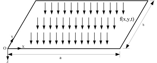
All loading points of distributed random load are completely correlative when all loading points of distributed random load are completely independent when and, part of loading points of distributed random load is correlative when which is the common situation. Especially, when correlation of distributed random load is non-spatial, the coherence function is or , and , the auto-spectral density at every spatial point is, and the cross-spectral density is For example, if coherence function of distributed random load is is auto-power spectrum density of the load, and its cross-spectral density function is the points of distributed random load will be partially coherent, and the statistical features of the load will only be related to the displacement in the space and will satisfy that ; and can be obtained when , .
2.3. A fast algorithm based on multi-dimensional Legendre orthogonal polynomials
There are five variants in plane-distributed random load applied on thin plates. To determinate , hypothetically and are defined within a certain range, auto-power spectrum density is a continuous function of and , the real and the imaginary parts of both and are also continuous functions. After projecting these continuous functions onto orthogonal basis functions, their optimal approximation is found as:
where .
where is a four-dimensional Legendre orthogonal polynomial, which is defined as a basis function. Therefore:
where .
The response cross-power spectrum density between points and is:
Given that:
Hence:
Fitting with certain precision requires an order number of , which can be written in matrices as:
When and , it yields the auto-power spectrum density of response.
Based on Eq. (19), represents the structural response in frequency domain under distributed harmonic load, . For every discrete , the orthogonal polynomial’s coefficients for fitting can be computed and structural response under harmonic load can be constructed with the coefficients and two-dimensional basis functions. According to the superposition of linear structures, linearly superimposing the responses of the structure under distributed harmonic load can finally lead to response power spectrum density of the structure. In this way, structural responses under distributed random load can be represented as responses in the frequency domain of the structure under determinate distributed harmonic load. According to the deduction above, this method takes all coupling items of the vibration frequency into consideration, which therefore makes it an accurate algorithm. The method is named pseudo-excitation method for two-dimensional distributed random loads.
If the distributed random load is linearly distributed at the position of elastic thin plate, the cross-spectral density function of any two points, and , can be described as . The algorithm above can be rewritten as:
Then the variant number of is reduced to three. For a determinate , within a certain range, it can be obtained as:
Finally, it can be simplified as:
where:
Based on the Eq. (26), represents structural response in frequency domain under distributed harmonic load, Similarly, for every discrete the orthogonal polynomials’ coefficients for fitting can be computed and structural response under harmonic load can be constructed by one-dimensional basis functions. According to the superposition of linear structures, linearly superimposing responses of the structure under linearly distributed harmonic load can finally lead to response power spectrum density of the structure. Simplified computation under linearly distributed random load is an extreme case of that under plane-distributed random load.
2.4. Comparison with regular algorithm in the computation speed
Computation of response in frequency domain under two-dimensional distributed random load is conducted with CQC, SRSS and the fast algorithm proposed in this paper. It is assumed that and are both known. Moreover, the former orders of modes are involved in the computation, and the three methods have the same number of discrete points in frequency domain. The algorithm employed to integrate is Gauss-Legendre integral formula as [24], where represents Gauss points in the interval and are Gauss coefficients corresponding to . Based on this formula, Gauss double integral formula is established as , where and are Gauss points in intervals and respectively; and and are Gauss coefficients corresponding to and respectively. Furthermore, Gauss quadruple integral formula is given that the number of Gauss points in every interval is the same .
Low computation efficiency mainly results from large amount of multiplication. The total number of multiplication for every discrete point in frequency domain with CQC method is ; it’s with SRSS method; with fast algorithm it is , where is the order of orthogonal polynomials required for fitting .
Table 1Comparison of the calculated amount of three methods (unit: number of multiplication)
Parameters | CQC | SRSS | Fast algorithm |
5, 5, 5, 16 | 1565000 | 62600 | 21600 |
5, 5, 10, 16 | 2500250 | 1000100 | 81600 |
10, 10, 10, 81 | 4.0004E+8 | 4.0004E+6 | 1.6524E+6 |
10, 10, 20, 81 | 6.40004E+9 | 6.40004E+7 | 6.5124E+6 |
As revealed in Table 1, the fast algorithm requires far less multiplication than CQC; and the smaller is, the more efficient the fast algorithm becomes. Generally speaking, the number of Gauss points that computation requires grows larger as gets bigger. Consequently, the fast algorithm is always more efficient than CQC and SRSS.
2.5. Computation instruction
Computation steps are as follows:
1) Calculate and . Their analytical solutions can be employed for typical structures. As for complex structures, can be obtained by finite element method.
2) Decompose in orthogonal domain and gain coefficients for fitting orthogonal polynomials.
3) Compute for every discrete points in frequency domain.
4) Conduct linear superposition based on Eq. (21) or (25), and obtain final results.
In summary, the fast algorithm for solving the problem of random response of elastic thin plate under distributed random load has two key steps. First, it projects the function of the cross power spectrum function onto orthogonal basis of multi-dimension Legendre polynomial and calculates the projection coefficient. Second, it calculates harmonic response under harmonic distributed load formed by the orthogonal basis function. In fact, it converts random response problem into a harmonic response problem, and harmonic response calculation is much easier than random response calculation. The fast algorithm applies to regular thin elastic plate and simple elastic structure, and it will be suitable for complicated structure after modification.
3. Simulation example
An elastic rectangular thin plate of homogeneous material with four simply supported edges is taken as the structure model. It has 1 m length, 0.6 m width, and 0.02 m thickness. The elastic modulus , density , Poisson's ratio is 0.3, modal damping ratio is 0.02, and number of finite elements is 240. The natural frequencies of the model are listed in Table 2. is a two-dimensional distributed random load, and represents the cross-spectral density of any two points.
Table 2First eight orders of the plate model
Orders | 1 | 2 | 3 | 4 | 5 | 6 | 7 | 8 |
Natural frequencies (Hz) | 183.88 | 326.85 | 565.75 | 588.29 | 720.27 | 898.67 | 941.63 | 1252.02 |
Example 1:
In this example, computation results of the fast algorithm and Nastran are compared, and efficiency is assessed. Due to incapability of defining coherence of distributed random load, Nastran can only compute distributed random load of complete coherence. Therefore, distributed random load in this example is set as complete coherence, and its power spectrum density is unit flat-spectrum.
The first eight orders are taken into computation. The order of orthogonal fitting is 1, and the number of Gauss points is 10. Frequency span is 1000 Hz, and frequency resolution is 1 Hz. Time consumed for computation is listed in Table 3. The power spectrum density line of acceleration at Node 125 of finite element model is displayed in Figures 2 and 3.
Table 3Comparison of time consumed
Algorithm | CQC | SRSS | Fast algorithm | Nastran |
Time consumed (s) | 19505.4 | 3733.3 | 485.047 | 478.6 |
Response at Node 125 of finite element model is computed with CQC, SRSS, the fast algorithm method and Nastran, under the same other conditions. As shown in Table 3, the fast algorithm is far more efficient than CQC and SRSS, and equivalent to that of Nastran (time consumed for computation includes time for computing coefficients of orthogonal polynomials).
Fig. 2The acceleration power spectrum density response result at Node125 with the finite element method
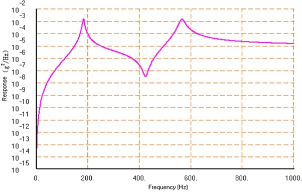
Fig. 3Comparison of the acceleration power spectrum density result at Node 125 with four methods
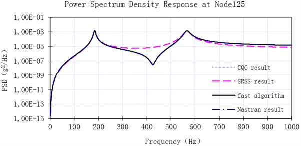
Figures 2 and 3 show that result of the fast algorithm is almost the same as that of Nastran, except the slight difference ranging from 900 Hz to 1000 Hz. It is due to different modal truncation. They also manifest that result of SRSS, displayed as pink dotted line, has some errors which are quite large at some points. These errors get even larger when damping ratio gets higher or modes become closer. The errors between the acceleration power spectrum density at natural frequencies produced by CQC, SRSS, the fast algorithm and Nastran are listed in Table 4. According to Table 4, the fast algorithm has the same result as CQC, and it is fairly close to the result of Nastran, while SRSS result shows great error.
Table 4Comparison between CQC, SRSS, the fast algorithm, and Nastran
Error types | Relative error between CQC and Nastran | Relative error between SRSS and Nastran | Relative error between fast algorithm and Nastran |
0.827 % | 1.853 % | 0.827 % | |
1.112 % | 13.922 % | 1.112 % |
Example 2:
In this example, the distributed random excitation is partially coherent, and the cross power spectrum density of distributed random load is defined as above. Derived from formula of Example 2, it is obtained that: , and .
Any two points are partially coherent when . First eight orders of modes are taken into computation. The orders of orthogonal fitting are , and the number of Gauss points is 10. The start frequency is 100 Hz, and stop frequency 400 Hz. Under the same other conditions, computation is conducted with CQC, SRSS, the new method and Nastran. The efficiency of computation is demonstrated in Table 5.
Table 5Comparison of three methods in computation
Algorithm | CQC | SRSS | Fast algorithm | Nastran |
Time consumed (s) | 523847 | 40104.8 | 11231.5 | Not applicable |
Table 5 further proves excellent efficiency of the fast algorithm. Fig. 4 illustrates the power spectrum density of response at Node 125 computed with these three methods, and errors are listed in Table 6. The largest error between SRSS and CQC is above 20 %, because of leaving cross items of mode shapes out. The fast algorithm possesses the same high precision as CQC, as shown in Figure 4.
Fig. 4Comparison of the acceleration power spectrum density result at Node 125 with the three methods
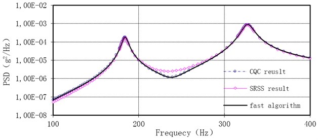
Table 6Computational errors of different methods
Error type | Relative error between CQC and SRS | Relative error between fast algorithm and SRSS | Relative error between fast algorithm and CQC |
Largest relative error | 24.97 % | 24.97 % | 6.357E-8 |
4. Conclusions
This paper proposes a fast algorithm for the calculation of structural response power spectrum density of thin plates under either one or two dimensional distributed random load. According to the simulation results of completely coherent two-dimensional distributed random load and partially coherent two-dimensional distributed random load, it is concluded that the proposed algorithm is fast as well as precise. Its efficiency is far higher than that of both CQC and SRSS. It is programmed for computation of structural responses in the frequency domain under two-dimensional distributed random load that is completely coherent, partially coherent or altogether incoherent. The efficiency is highly improved, and the precision is also guaranteed. It facilitates the computation of responses under distributed random load in engineering. In addition, it establishes a basis for the subsequent identification of distributed random load.
References
-
Zhang Fang, Qin Yuantian, Deng Jihong. Research of identification technology of dynamic load distributed on the structure. Journal of Vibration Engineering, Vol. 19, Issue 1, 2006, p. 81-85.
-
Cameron W., Coates Thamburaj P. Inverse method using finite strain measurement to determine flight load distribution functions. Journal of Aircraft, Vol. 45, Issue 2, 2008, p. 366-370.
-
Coates C. W., Thamburaj P., Kim C. An inverse method for selection of Fourier coefficients for flight load identification. Proceedings of the 46th Annual AIAA/ASME/ASCE/AHS Structures, Structural Dynamics and Mechanics Conference, AIAA, Reston, 2005, p. 18-21.
-
Lin J. H., Guo X. L., Zhi H., Howson W. P. Computer simulation of structural random loading identification. Computers and Structures, Vol. 79, Issue 4, 2001, p. 375-387.
-
K. Soyluk. Comparison on random vibration methods for multi-support seismic excitation analysis of long-span bridges. Engineering Structures, Vol. 26, Issue 11, 2004, p. 1776-1778.
-
Lin J. H., Williams F. W. Computation and analysis of multi-excitation random seismic responses. Engineering Computations, Vol. 9, Issue 5, 1992, p. 561-574.
-
Xue S. D., Li M. H., Cao Z., Zhang Y. G. Random vibration analysis of lattice shell subjected to multi-dimensional earthquake inputs. Proc. Int. Conf. on Advances in Structural Dynamics, Elsevier, 2000, p. 777-784.
-
Jiang Jinhui, Chen Guoping, Zhang Fang. Fast algorithm for structural frequency domain response subjected to one-dimension distributed random load. Journal of Vibration and Shock, Vol. 29, Issue 8, 2010, p. 55-59.
-
P. Sniady, S. Biernat, R. Sieniawska, S. Zukowsky. Vibrations of the beam due to a load moving with stochastic velocity. Probabilist. Eng. Mech., Vol. 16, Issue 1, 2001, p. 53-59.
-
S. S. Law, X. Q. Zhu. Bridge dynamic responses due to road surface roughness and braking of vehicle. J. Sound Vibration, Vol. 282, 2005, p. 805-830.
-
W. X. Zhong. Review of a high-efficiency algorithm series for structural random responses. Prog. Nat. Sci., Vol. 6, Issue 3, 1996, p. 257-268.
-
M. F. Dimentberg, B. Ryzhik, L. Sperling. Random vibrations of a damped rotating shaft. Journal of Sound and Vibration, Vol. 279, 2005, p. 275-284.
-
Zhou X. Y., Yu R. F. Mode superposition method of non stationary seismic responses for non classically damped linear systems. Journal of Earthquake Engineering, Vol. 12, Issue 3, 2008, p. 597-641.
-
J. H. Lin, Y. H. Zhang, Y. Zhao. Pseudo excitation method and some recent developments. Proceedings of the Twelfth East Asia-Pacific Conference on Structural Engineering and Construction, Hong Kong, January, 2011, p. 2453-2458.
-
A. D. Kiureghian, A. Neuenhofer. Response spectrum method for multi-support seismic excitations. Earthquake Engrg. and Struct. Dynamics, Vol. 21, Issue 8, 1992, p. 713-740.
-
H. Z. Ernesto, E. H. Vanmarcke. Seismic random vibration analysis of multi-support structural systems. ASCE J. Eng. Mech., Vol. 120, 1994, p. 1107-1128.
-
Wei Guo, Zhiwu Yu. Pseudo excitation method based on multiple degree of freedom modal equation. Advanced Materials Research, 2012, p. 317-320.
-
Yu R. F., Wang L., Liu H., Zhou X. Y. The CQC3 method for multi component seismic responses of non-classically damped irregular structures. American Structures Congress, New York, 2005.
-
Q. Gao, J. H. Lin, W. X. Zhong, W. P. Howson, F. W. Williams. Propagation of partially coherent non-stationary random waves in viscoelastic layered half-space. Soil Dynamics and Earthquake Engineering, Vol. 28, Issue 4, 2008, p. 305-320.
-
Zhichao Zhang, Yahui Zhang, Jiahao Lin, Yan Zhao, W. P. Howson, F. W. Williams. Random vibration of a train traversing a bridge subjected to traveling seismic waves. Engineering Structures, Vol. 33, Issue 12, 2011, p. 3546-3558.
-
Y. L. Xu, N. Zhang, H. Xia. Vibration of coupled train and cable-stayed bridge systems in cross winds. Eng. Struct., Vol. 26, Issue 10, 2004, p. 1389-1406.
-
Li J., Liao S. T. Response analysis of stochastic parameter structures under non-stationary random excitation. Comput. Mech., Vol. 27, Issue 1, 2001, p. 61-68.
-
Lin J. H., Zhao Y., Zhao Y. H. Accurate and highly efficient algorithms for structural stationary/non-stationary random responses. Comput. Methods Appl. Mech. Eng., Vol. 191, 2001, p. 103-111.
-
Sansone G. Orthogonal Functions. English Ed., New York, Dover, 1991.
-
Charles C. Dyer, Peter S. S. Ip. An Elementary Introduction to Scientific Computing. Division of Physical Sciences, University of Toronto at Scarborough, January 2000.
About this article

The research described in this paper was supported by the Fundamental Research Funds for the Central Universities No. NS2012080, the Aeronautical Science Foundation of China under Grant No. 2012ZA52001, and Research Fund for the Doctoral Program of Higher Education of China No. 20123218120005.
