Abstract
In recent years, condition monitoring and fault diagnosis of hydraulic servo systems has attracted increasing attention. However, few studies have focused on the performance assessment of these systems. This study proposes a performance assessment method based on a bi-step neural network and an autoregressive model for a hydraulic servo system; the performance is quantized by the performance confidence value (CV). First, a fault observer based on a radial basis function (RBF) neural network is designed to estimate the output of the system and calculate the residual error. Second, the corresponding adaptive threshold is generated by using another RBF neural network during system operation. Third, the difference value between the coefficients of the autoregressive model for the generated residual error and the adaptive threshold is obtained, and the Mahalanobis distance (MD) between the most recent difference (unknown conditions) and the constructed Mahalanobis space by using samples under normal conditions is calculated. Then, the condition of the system can be determined by normalizing the MD into a CV. The proposed method was further validated for three types of faults, and data were obtained using a simulation model. The experimental analysis results show that the performance of hydraulic servo systems can be assessed effectively by the proposed method.
1. Introduction
Hydraulic servo systems are widely used for industrial applications where heavy objects need to be manipulated or large forces need to be exerted, for example, in pick-and-place robots. Furthermore, they are used in the aerospace field, for examples, to position aircraft control surfaces, in flight simulators, and in missiles. Such systems are used in a large variety of critical applications, and therefore, it is very important to ensure that they operate normally and efficiently. Furthermore, it is important to carry out proper and efficient maintenance of such systems when they operate abnormally. In most cases, the decision to conduct maintenance is based on a performance confidence value ranging between zero and one that is obtained through a performance assessment. Therefore, accurate performance assessment is essential for the efficient maintenance of hydraulic servo systems.
Many studies have previously focused on the fault detection and diagnosis of hydraulic servo systems, and the use of observer models and other types of models has been proposed for this purpose. Liu proposed a two-stage radial basis function (RBF) neural network model to realize failure detection and fault localization. He studied a fuzzy auto-regressive with extra inputs (ARX) model structure and the corresponding fault feature extraction and proposed a fault feature extraction approach based on this model for a hydraulic system. However, both of these studies focused on the fault detection and fault localization of a hydraulic servo system, which is not sufficient for conducting efficient maintenance of hydraulic servo systems. Jelali studied performance assessment with a focus on typical mechanical components such as bearings and gears or the control systems. Similarly, Yu proposed bearing performance degradation assessment using locality-preserving projections and Gaussian mixture models, whereas Pan proposed bearing performance degradation assessment based on improved wavelet packet decomposition (IWPD) and support vector data description (SVDD). However, the performance degradation assessment methods proposed in these studies for typical mechanical components are not suitable for hydraulic servo systems. Basically, few studies have focused on performance assessment methods for hydraulic servo systems.
In this study, a performance assessment method based on a bi-step neural network and an autoregressive (AR) model is proposed for hydraulic servo systems. The bi-step neural network comprises two RBF neural networks. The first one is used to track the actual system and generate the residual error, and the second one is used to synchronously output the corresponding adaptive threshold. Then, the AR model is applied to the residual error and adaptive threshold, and the AR model coefficients are used to assess the performance of the hydraulic servo system. An AR model is a time sequence analysis method whose parameters provide important information about the system condition, and an accurate AR model can reflect the characteristics of a dynamic system. Finally, the difference value between the coefficients of the autoregressive model for the generated residual error and the adaptive threshold is obtained, and the MD between the most recent difference (unknown conditions) and the constructed Mahalanobis space by using samples under normal conditions is calculated and normalized. The result of the performance assessment, that is, the confidence value, can be used to make maintenance decisions. A simulation case study is used to validate the effectiveness of the proposed performance assessment method for the hydraulic servo system.
The remainder of this paper is organized as follows. In section 2, the simulation model of the hydraulic servo system is presented. In section 3, a detailed description of the proposed method is presented. In section 4, the results of the simulation experiment are presented and discussed.
2. Set up of the hydraulic servo system
The hydraulic servo system consists of an electrohydraulic servo valve, a cylinder, two electronic amplifiers, and a displacement sensor, a force sensor. The control loop includes a position feedback and a force feedback (see Fig. 1).
Fig. 1Closed-loop control system of hydraulic servo system
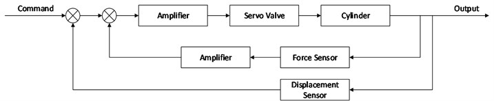
Fig. 2Control part in Simulink
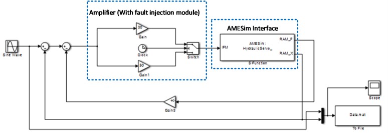
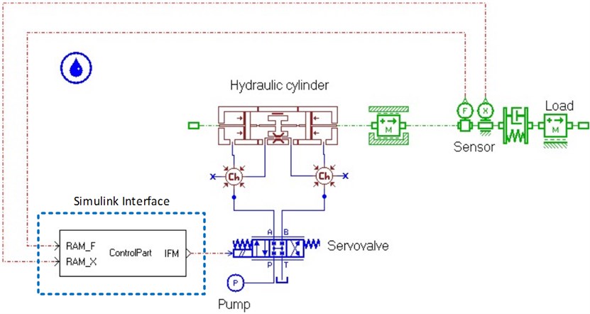
The simulation model of the hydraulic servo system is established by using Matlab Simulink and AMESim. The control part of the hydraulic servo system, which is established in Simulink environment, is shown in Fig. 2; the mechanical part of the hydraulic servo system is shown in Fig. 3. The mechanical part of the hydraulic servo system established in AMESim is converted to a Simulink S-Function, and the S-Function can be imported to Simulink. The physical parameters of the key components are described below.
Fig. 3Mechanical part in AMESim
2.1. Servo valve
The physical parameters of the servo valve are shown in Table 1.
Table 1Physical parameters of servo valve
SV00-1: All real parameters | Unit | Value |
Ports P to A flow rate at maximum valve opening | L/min | 75 |
Ports P to A corresponding pressure drop | bar | 100 |
Ports P to A critical flow number (laminar → turbulent) | null | 1000 |
Ports B to T flow rate at maximum valve opening | L/min | 75 |
Ports B to T corresponding pressure drop | bar | 100 |
Ports B to T critical flow number (laminar → turbulent) | null | 1000 |
Ports P to B flow rate at maximum valve opening | L/min | 75 |
Ports P to B corresponding pressure drop | bar | 100 |
Ports P to B critical flow number (laminar → turbulent) | null | 1000 |
Ports A to T flow rate at maximum valve opening | L/min | 75 |
Ports A to T corresponding pressure drop | bar | 100 |
Ports A to T critical flow number (laminar → turbulent) | null | 1000 |
Working density for pressure drop measurement | kg/m3 | 850 |
Working kinematic viscosity for pressure drop measurement | cSt | 60 |
Valve rated current | mA | 1 |
Valve natural frequency | Hz | 500 |
Valve damping ratio | null | 0.8 |
Deadband as fraction of spool travel | null | 0 |
2.2. Cylinder
Considering the injection of internal leakage fault, the cylinder consists of three hydraulic component design modules: 2 piston modules, 1 leakage and viscous friction module.
The physical parameters of the piston modules are shown in Table 2.
Table 2Physical parameters of piston modules
BAP11-1: All real parameters | Unit | Value |
Piston diameter | mm | 90 |
Rod diameter | mm | 30 |
Chamber length at zero displacement | mm | 150 |
The physical parameters of the leakage and viscous friction module are shown in Table 3.
Table 3Physical parameters of leakage and viscous friction module
BAF11-1: All real parameters | Unit | Value |
External piston diameter | mm | 90 |
Clearance on diameter | mm | 1e-05 |
Length of contact | mm | 30 |
2.3. Mass and displacement limit
The physical parameters of the mass and displacement limit module are shown in Table 4.
Table 4Physical parameters of mass and displacement limit module
MAS005-1: All real parameters | Unit | Value |
Mass | kg | 10 |
Coefficient of viscous friction | N/(m/s) | 5000 |
Coefficient of windage | N/(m/s)2 | 0 |
Coulomb friction force | N | 1000 |
Stiction force | N | 1000 |
Lower displacement limit | m | -0.15 |
Higher displacement limit | m | 0.15 |
Inclination (+90 port 1 lowest, –90 port 1 highest) | degree | 0 |
2.4. Displacement sensor
The physical parameters of the displacement sensor are shown in Table 5.
Table 5Physical parameters of displacement sensor
DT000-1: All real parameters | Unit | Value |
Offset to be subtracted from displacement | m | 0 |
Gain for signal output | 1/m | 1 |
2.5. Force sensor
The physical parameters of the force sensor are shown in Table 6.
Table 6Physical parameters of force sensor
FT000-1: All real parameters | Unit | Value |
Offset to be subtracted from force | N | 0 |
Gain for signal output | 1/N | 1 |
3. Performance assessment method using bi-step neural network and autoregressive model
Performance assessment is advantageous because its result, namely, the confidence value, can be applied in models such as the time-dependent proportional hazards model as a performance indicator, and this is essential for deciding whether the hydraulic servo system needs to be maintained. Fig. 4 shows the particular approach adopted in this study.
Fig. 4Performance assessment based on bi-step neural network and AR model
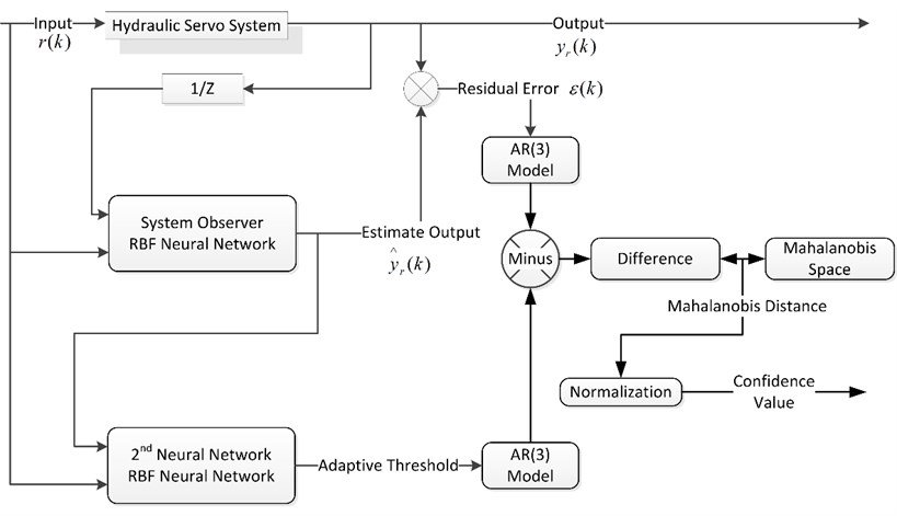
Compared with linear methods, nonlinear methods such as a neural network, fuzzy models, and hybrid models show better sensitivity to abnormal states of hydraulic servo system. As shown in Fig. 4, an RBF neural network is used because of its nonlinear mapping capability and training efficiency. An observer based on the RBF neural network is used to estimate the output of the real system. The residual error between the system output and the output estimated by the observer can be used for performance assessment. If it is close to zero, the hydraulic servo system is considered to be in a normal condition; otherwise, the system is considered to be performing poorly. The residual error is derived without considering the influence of noise and model errors; this might lead to non-zero residuals and, in turn, poorer performance. Therefore, a threshold is introduced to assess the performance of the hydraulic servo system. This threshold directly affects the performance assessment: if it is too high, it may lead to better performance than under real conditions, whereas if it is too low, it may lead to worse performance than under real conditions. Therefore, the threshold needs to be adaptively adjusted. Another neural network is designed to generate the adaptive threshold. The input signals and the estimated output from the observer are input into the RBF neural network to obtain the adaptive threshold synchronously. Considering that the parameters of the AR model are very sensitive to variations in the conditions, the coefficients of the AR model are extracted from the residual error and adaptive threshold to assess the performance of the hydraulic servo system. The order of the AR model is selected using the Akaike information criterion (AIC), and the coefficient estimates are obtained by using the Burg method. Then, the value of difference between the coefficients of the residual error and the adaptive threshold is calculated, and the Mahalanobis space is constructed by the differences that represent “normal” conditions. Finally, the MD, between the most recent difference and the constructed Mahalanobis space, is calculated and, in turn, normalized into a CV.
3.1. Observer model based on 1st RBF neural network
Suppose that the hydraulic servo system can be described as:
where , , and denote the state vector, output vector, input vector, and failure vector, respectively, and and are the nonlinear vector functions.
The state observer is defined as:
The state error is defined as:
If when or , then Eq. (2) is called the fault observer of Eq. (1).
To effectively describe the nonlinearity in the hydraulic servo system, the RBF neural network shown in Fig. 4 is adopted as a fault observer, where and denote the output and input of the system, respectively, and is the estimated output of the fault observer.
The adopted RBF neural network consists of three layers: the input layer, the hidden layer and output layer. The input layer of an RBF neural network is constituted by input nodes; the second layer is hidden layer, and the number of nodes can be determined as required; the third layer is output layer. The output of an RBF neural network is:
Normally, a Gaussian function is chosen as the radial basis function:
where the input vector is the independent variable vector of Gaussian function; is the constant vector, namely, the center of radial basis function; and is the radial basis function.
For the training of the RBF neural network observer, the mean squared error goal is set to 0.08; the spread of radial basis function, 2; and the maximum number of neurons, 50, respectively.
The residual error is generated based on a comparison between the actual and the estimated system response. The latter is generated by the RBF neural network observer. The residual error is defined as the difference between the actual and the estimated output:
Under normal conditions, the residual error is only due to the influence of noise and modeling errors, and it is close to zero. The residual error in this case is defined as the baseline residual and is denoted as . However, in the presence of some faults, the residual error deviates from zero in characteristic ways.
3.2. Adaptive threshold generation based on 2nd RBF neural network
The main factors influencing the threshold of the hydraulic servo system are the system input, system output, and some random factors such as the modeling error, random disturbance, random noise, and parameter drift. Considering that the observer is very robustness, the authors assume that the threshold only depends on the system input and system output. Then, the mapping relationship among the system input, system output, and threshold can be established. Another RBF neural network is selected to fit this relationship because RBFs have good nonlinear mapping capability and training efficiency. Like the RBF neural network mentioned above, the RBF neural network that is used to generate threshold also contain three layers, and the radial basis function is Gaussian function.
The second RBF neural network is trained by using the system input and estimated output as the input training datasets and the expected threshold of the system as the output training datasets. The expected threshold of the system depends on the baseline threshold and influencing factors (see Eq. (7)):
In Eq. (10), is the baseline threshold generated by the first neural network observer and is the correction coefficient.
Regarding the RBF network training process for the adaptive threshold generation, the mean squared error goal, the spread of radial basis functions, and the maximum of neurons are defined as 0.001, 2, and 30, respectively.
3.3. Coefficient extraction of AR model
An AR model is simply a linear regression of the current value against one or more prior values of the series. An AR model of order is defined as:
where are the AR coefficients and is a Gaussian white-noise series with zero mean and variance . An AR model is a time sequence analysis method whose parameters contain important information about the system condition, and it has been successfully applied to the fault diagnosis in recent years. In fact, in view of the stationarity in the input signal of hydraulic servo systems, the spectrum of the AR moving average process can be represented purely in terms of AR coefficients, without the need of computing the moving average model coefficients. The advantage of the AR model is: differing from a moving average model (the moving average part of ARMA), its parameters can be determined by solving a linear set of equations. Generally, an AR model requires far fewer coefficients than the corresponding moving average model, and thus, it is more effective for those signals with sharp peaks (e.g. residual error and adaptive threshold).
The selection of the order of the AR model is a crucial step because spurious spectral peaks and general statistical instability will be caused if the order is too large, whereas smoothed spectral peaks will be cause if the order is too small. In this study, the order is selected based on the AIC. The AIC, which reflects the effect of the spectral variance due to the increase in model order and prediction errors computed in estimating the AR coefficients, is given by:
In this study, an order of 3 is selected for the AR model.
When the signal is stationary, the coefficients of the AR model are most commonly determined either by using the autocorrelation (second-order statistical characteristic) of the signal or by solving the Yule-Walker equations, and the latter can be done by several methods. The two most commonly used methods are the Levinson-Durbin recursion (LDR) algorithm and the Burg (maximum entropy) method (BM). Both ARMA and ARIMA models can be applied to both stationary and non-stationary signals, but the increasing computation time is needed. Considering the input command of hydraulic servo system is stationary signal, an AR model is sufficient for the purpose of performance assessment. In this study, the Burg method is adopted.
3.4. MD calculation and normalization
MD, introduced by P.C. Mahalanobis in 1936, is a multivariate generalized measure used to determine the distance of a data point to the mean of a cluster. It is measured in terms of the standard deviations from the mean of the samples and provides a statistical measure of how well the unknown data set matches with the ideal one. The advantage of the MD is that it is sensitive to the inter-variable changes in the reference data. In this study, the MD is used to assess the performance of hydraulic servo systems.
The MD is calculated as follows:
a) Calculate the mean for each characteristic in a normal dataset as:
b) Calculate the standard deviation for each characteristic:
c) Normalize each characteristic, form the normalized data matrix , and take its transpose :
d) Form the correlation matrix for the normalized data. Calculate the matrix elements as follows:
e) Finally, calculate the MD as:
As mentioned above, the order of the AR model is 3 in this study. The AR(3) process is given by Eq. (15), where , and are the coefficients of the process and is an independent and identically distributed random noise process with zero mean and variance :
The AR(3) model divides into two parts: deterministic part and stochastic part. The former is determined by the expectation of , that is:
Therefore, the coefficients , and reflect the system performance.
Suppose that the residual error contains epochs, and one spot in three dimensions is extracted from epochs. Then, spots are extracted from the residual error. Similarly, spots are extracted from the adaptive threshold.
Under normal conditions, the value of the difference between the coefficients of the residual error and the coefficients of the adaptive threshold contains spots, and these spots are denoted as follows:
where and
are the coefficients of the AR(3) model extracted from the residual error and the adaptive threshold, respectively, under normal conditions. Below, is used to construct the Mahalanobis space as the benchmark reference.
Similarly, spots can be extracted from the residual error and adaptive threshold under unknown conditions or the most recent measurement. These spots are denoted as follows:
where and
are the coefficients of the AR(3) model extracted from the residual error and the adaptive threshold under unknown conditions.
By using the method above, the MD can be obtained. As aforementioned, the Mahalanobis space is constructed by using the differences between the coefficients of the AR model for the generated residual error and the adaptive threshold under normal conditions. Then, the distance between and the constructed Mahalanobis space, which is defined as Mahalanobis distance, actually indicates how far the most recent feature vector deviates from normal condition. Hence, the degradation trend can be visualized by the curve of MD over time. As the MD increases, the performance degradation becomes severer accordingly.
Then, the MD is normalized into [0, 1] as a confidence value (CV). The CV, representing the performance of a hydraulic servo system, can be formulated as below:
where is the MD and is a shape parameter. The MDs obtained from normal states are closer to the constructed Mahalanobis space, compared with those obtained from performance degradation or fault states. Meanwhile, the normalization function is a monotone decreasing function, thus, the CV will be higher as the system shows better performance.
4. Case study
4.1. Experimental design
A simulation model with fault injection modules was used to evaluate the proposed method. The hydraulic servo system consists of various components, as shown in Figs. 2 and 3. Statistical data of hydraulic servo system faults indicates that the main fault modes of these systems are electronic amplifier faults, actuator cylinder faults, leakage faults, and sensor faults. In this study, electronic amplifier fault, sensor fault and internal leakage fault were injected to the simulation model. The detail of fault injection is described below.
(1) Electronic amplifier fault injection
Electronic amplifier fault injection module is shown in Fig. 2. The parameters of normal amplifier and fault amplifier are shown in Table 7.
Table 7Parameters of electronic amplifier (Normal and Fault)
Gain of electronic amplifier | |
Normal | 50 |
Fault | 30 |
(2) Sensor fault injection
The physical parameters of fault sensor are shown in Table 8.
Table 8Physical parameters of fault sensor
DT000-1: All real parameters | Unit | Value |
Offset to be subtracted from displacement | m | 0 |
Gain for signal output | 1/m | 0.75 |
(3) Leakage fault injection
In order to compare the CVs of hydraulic servo system under different degradation level, slight leakage fault, moderate leakage fault and severe leakage fault were injected. The physical parameters of leakage fault are shown in Table 9, Table 10 and Table 11.
Table 9Physical parameters of slight leakage fault
BAF11-1: All real parameters | Unit | Value |
External piston diameter | mm | 90 |
Clearance on diameter | mm | 1 |
Length of contact | mm | 30 |
Table 10Physical parameters of moderate leakage fault
BAF11-1: All real parameters | Unit | Value |
External piston diameter | mm | 90 |
Clearance on diameter | mm | 1.1 |
Length of contact | mm | 30 |
Table 11Physical parameters of severe leakage fault
BAF11-1: All real parameters | Unit | Value |
External piston diameter | mm | 90 |
Clearance on diameter | mm | 1.2 |
Length of contact | mm | 30 |
The input signal for the simulation model of the hydraulic servo system is:
Faults were introduced into the actuator cylinder, electronic amplifier, and sensor. For data acquisition, a sampling rate of 10 is used; the simulation time is 600 s. Four tests were conducted, and the details of each test are shown in Table 12. The correction coefficient in this case is 0.2. Note that one spot was extracted from 50 epochs of residual error/adaptive threshold, and therefore, the confidence value contains 120 epochs.
Table 12Details of each test
Fault mode | Fault injection time | |||
Time | Raw data epoch | CV epoch | ||
Test 1 | Normal | |||
Test 2 | Electronic amplifier fault | 200 s | 2000th epoch | 40th epoch |
Test 3 | Sensor fault | 200 s | 2000th epoch | 40th epoch |
Test 4 | Leakage fault Clearance 1 mm | 150 s | 1500th epoch | 30th epoch |
Leakage fault Clearance 1.1 mm | 300 s | 3000th epoch | 60th epoch | |
Leakage fault Clearance 1.2 mm | 450 s | 4500th epoch | 90th epoch | |
4.2. Procedure and details of the test
The approach adopted in this study is shown in Fig. 4, and more details and the test procedure are shown in Fig. 5. In this flowchart, the authors take test 4 as an example. The others tests were conducted similarly.
4.3. Comparison of test results
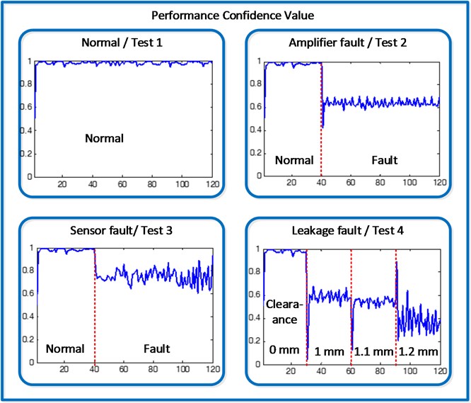
The performance confidence values of the hydraulic servo system as calculated by using the proposed method are shown in Fig. 6. This value indicates the performance of the system. The curve of this value over time is representative of the degradation of the hydraulic servo system. In test 1, no fault was injected into the system; therefore, the system operated normally, with a performance confidence value of ~0.9. In test 2, an electronic amplifier fault was injected into the model at 200 s; then, it was observed that between 1 and 200 s (1st to 40th epochs in figure), the performance confidence value fluctuated around 0.9, before it decreased abruptly at 200 s (40th epoch in figure). In test 3, a sensor fault was injected, then, at 200 s (40th epoch in figure), the performance confidence value decreased to 0.7. In test 4, three internal leakage faults were injected into the cylinder, with different fault severity; at 150 s (30th epoch in figure), an internal leakage fault with clearance diameter of 1mm was injected, and the performance CV decreased to 0.6; at 300 s (60th epoch in figure), a severer leakage fault with clearance diameter of 1.1 mm was injected to the cylinder, then, the performance CV decreased to ~0.55; at last, the performance CV decreased to ~0.4 as a more severer leakage fault was injected. These test results indicate that the performance confidence value can not only detect the occurrence of faults but also reflect the degradation in performance. Thus, the performance confidence value obtained by using the proposed method can serve as an effective index for determining whether maintenance needs to be carried out.
Fig. 5Step-by-step diagram of the proposed performance assessment method
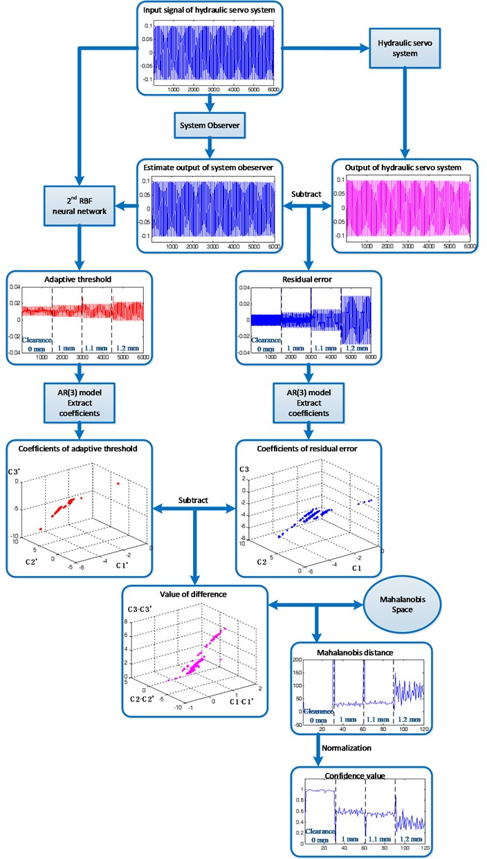
Fig. 6Comparison of results for each fault in the hydraulic servo system
5. Conclusions
This study develops a performance assessment method for a hydraulic servo system based on a bi-step neural network and an AR model. In the second RBF neural network, the threshold used to assess performance can be adaptively adjusted according to a variety of influencing factors. Furthermore, the performance confidence value can be calculated from the coefficients extracted using the AR model. Experimental results indicate that the proposed method can detect faults of several components, and it can clearly reveal the fault degrees. The proposed method could be further extended and improved to make it applicable to the performance assessment of other nonlinear systems such as control components in an aircraft environment control system, because the issues in such systems are similar to those in hydraulic servo systems. Furthermore, fault classification might be possible if this method is combined with a signal processing method such as wavelet package decomposition.
References
-
Jiang Bin, F. Chowdhury. Observer-based fault diagnosis for a class of nonlinear systems. Paper presented at the American Control Conference, Vol. 5676, 2004, p. 5671-5675.
-
Dragan Djurdjanovic, Jay Lee, Jun Ni. Watchdog agent – an infotronics-based prognostics approach for product performance degradation assessment and prediction. Advanced Engineering Informatics, Vol. 17, Issue 3-4, 2003, p. 109-125.
-
Yuan Hang, Lu Chen, Wang Zhaobing, Fan Huanzhen. Fault prediction of control components in aircraft environmental control system based on adaptive threshold. Lecture Notes in Information Technology, Vol. 14, 2012, p. 83-88.
-
Xiangyu He. Fault diagnosis approach of hydraulic system using Farx model. Procedia Engineering, Vol. 15, 2011, p. 949-953.
-
Liu Hongmei, Lu Chen, Hou Wenkui, Wang Shaoping. An adaptive threshold based on support vector machine for fault diagnosis. 8th International Conference on Reliability, Maintainability and Safety, ICRMS 2009, 2009, p. 907-911.
-
Andrew K. S. Jardine, Daming Lin, Dragan Banjevic. A review on machinery diagnostics and prognostics implementing condition-based maintenance. Mechanical Systems and Signal Processing, Vol. 20, Issue 7, 2006, p. 1483-1510.
-
Mohieddine Jelali. An overview of control performance assessment technology and industrial applications. Control Engineering Practice, Vol. 14, Issue 5, 2006, p. 441-466.
-
Cheng Junsheng, Yu Dejie, Yang Yu. A fault diagnosis approach for roller bearings based on Emd method and Ar model. Mechanical Systems and Signal Processing, Vol. 20, Issue 2, 2006, p. 350-362.
-
H. Khan, Seraphin C. Abou, N. Sepehri. Nonlinear observer-based fault detection technique for electro-hydraulic servo-positioning systems. Mechatronics, Vol. 15, Issue 9, 2005, p. 1037-1059.
-
Wenbin Li, Jianyu Zhang, Lingli Cui, Lixin Gao, Feibin Zhang. Application of multiwavelet adaptive threshold denoising in the fault diagnosis of gearbox. 2011 Third International Conference on Measuring Technology and Mechatronics Automation (ICMTMA), 2011, p. 551-554.
-
Linxia Liao, Jay Lee. A novel method for machine performance degradation assessment based on fixed cycle features test. Journal of Sound and Vibration, Vol. 326, Issue 3-5, 2009, p. 894-908.
-
Hong-Mei Liu, Shao-Ping Wang, Ping-Chao Ouyang. Fault diagnosis in a hydraulic position servo system using Rbf neural network. Chinese Journal of Aeronautics, Vol. 19, Issue 4, 2006, p. 346-353.
-
M. Montanari, F. Ronchi, C. Rossi, A. Tilli, A. Tonielli. Control and performance evaluation of a clutch servo system with hydraulic actuation. Control Engineering Practice, Vol. 12, Issue 11, 2004, p. 1369-1379.
-
Yuna Pan, Jin Chen, Lei Guo. Robust bearing performance degradation assessment method based on improved wavelet packet – support vector data description. Mechanical Systems and Signal Processing, Vol. 23, Issue 3, 2009, p. 669-681.
-
Emanuel Parzen. Autoregressive Spectral Estimation. Handbook of Statistics. Elsevier, Editors: D. R. Brillinger, P. R. Krishnaiah, 1983, p. 221-247.
-
S. Poyhonen, P. Jover, H. Hyotyniemi. Signal processing of vibrations for condition monitoring of an induction motor. First International Symposium on Control, Communications and Signal Processing, 2004, p. 499-502.
-
Doo Seung Ho, Ra Won-Sang, Yoon Tae Sung, Park Jin Bae. Fast time-frequency domain reflectometry based on the Ar coefficient estimation of a chirp signal. American Control Conference, 2009, p. 3423-3428.
-
Ahmet Soylemezoglu, S. Jagannathan, Can Saygin. Mahalanobis Taguchi system (Mts) as a prognostics tool for rolling element bearing failures. Journal of Manufacturing Science and Engineering, Vol. 132, Issue 5, 2010, p. 051014.
-
Xiaofang Wang, Qinghua Li, Jun Li. An adaptive threshold segmentation method based on Bp neural network for paper defect detection. 2011 IEEE 2nd International Conference on Software Engineering and Service Science (ICSESS), 2011, p. 405-408.
-
Xiyang Wang, Viliam Makis. Autoregressive model-based gear shaft fault diagnosis using the Kolmogorov–Smirnov test. Journal of Sound and Vibration, Vol. 327, Issue 3-5, 2009, p. 413-423.
-
Jianbo Yu. Bearing performance degradation assessment using locality preserving projections and Gaussian mixture models. Mechanical Systems and Signal Processing, Vol. 25, Issue 7, 2011, p. 2573-2588.
About this article

This research is supported by the National Natural Science Foundation of China (Grant No. 61074083, 50705005, and 51105019), and by the Technology Foundation Program of National Defense (Grant No. Z132010B004).
