Abstract
Matching pursuit (MP) with pulse atoms adaptively matches the pulse components in the vibration signals of faulty rolling bearings, and the atomic parameters correspond with the fault features. However, the decomposition of matching pursuit with pulse atoms (MP_PA) is equivalent to searching extremum of multimodal function with considerably large calculation. Therefore, a niching particle swarm optimization, which has high global convergence ability and convergence speed, was combined with the segment and joint method to simplify MP_PA, and the efficiency was greatly improved. The parameters of pulse atom which contain almost all the information of pulse nearly completely reflect the status of bearings, by them not only the characteristic defect frequency could be extracted, but also the other features such as frequency center, damping coefficient and so on. The random in the motion of the bearings makes the pulses in vibration signals be cyclostationary rather than purely periodic, thus by using cyclostationary statistics, more accurate characteristic defect frequency could be obtained. Followed by a comparison with wavelet transform (WT) and Empirical Mode Decomposition (EMD), the techniques based on parameters of pulse atoms and degree of cyclostationarity (DCS) provide precise and explicit characteristic defect frequency of the bearing with weak defect. At last, the multi features from DCS and atomic parameters were applied to identify the status of the measured bearings accurately. These results indicate that, due to the extraction of comprehensive and accurate fault features, and strong anti-interference ability, these techniques are appropriate to fault diagnosis of bearings.
1. Introduction
Rolling bearings are widely used in construction machinery, power station, spacecraft and other equipment, their conditions often directly affects the accuracy, reliability and lifetime of the entire system. Therefore, an accurate, efficient and intelligent fault diagnosis of rolling bearings is of great significance. Demodulated resonance technique [1], Wigner-Ville distribution (WVD) [2] and wavelet transform (WT) [3] are commonly used approaches for bearing diagnosis, however, they still have some drawbacks. For example, the resolutions are not high enough, and the appropriate frequency bands or decomposition levels often need to be selected manually, which requires the experienced diagnostic persons.
In recent years, matching pursuit [4] proposed by Mallat has been a powerful tool for non-stationary signal processing, considerable attempts have been made to apply MP in the fault diagnosis of rolling bearing [5, 6], gear [7]. Especially some researchers applied MP_PA [8] whose atoms correspond to fault features and attenuate in one side into the fault diagnosis of reciprocating machinery [9] and gear [10], etc. Because MP_PA adaptively selects the atom which matches pulse components with no intermediate process, it not only maximally reserves the intrinsic features of the signal, but also filters noises and interferential components, so that many successes have been achieved. MP_PA works perfectly because the pulse atoms (also named damped sinusoidal atom) match the pulse components. But solving MP_PA is a problem of searching the extremum of a complex, continuous and non-differentiable multimodal function [9], due to huge calculation, it often needs to resort to artificial intelligence algorithms [6], yet it is easy to be trapped into local optimal solutions. The niching particle swarm optimization (NPSO) [11-14] has received more attention in recent years due to the high global convergence ability and convergence speed which is more suitable for solving such sort of problems; consequently it is a good choice to employ NPSO to optimize MP_PA.
Existing studies are often based on the reconstructed signal by MP, and almost only one feature of characteristic defect frequency is extracted for fault diagnosis. In fact, the parameters of pulse atoms which correspond with fault features and almost contain all the information of pulses. If the features are extracted directly from these parameters, not only the process would be more direct and convenient, but also more comprehensive faulty information could be extracted. What’s more, the pulses of faulty bearings are cyclostationary rather than purely periodic [15]. Therefore, by the help of DCS [16], more accurate characteristic defect frequency could be acquired.
In order to diagnose the fault of rolling bearings automatically and efficiently, firstly, we used MP_PA which has been simplified by NPSO and the segment and joint method (SJ) to decompose the vibration signals of bearings, and then extracted characteristic defect frequency on the foundation of DCS, followed by a comparative analysis with wavelet envelope spectrum and EMD envelope spectrum of raw vibration signals. Finally, multi features, including the amplitude of characteristic defect frequency, frequency center, pulse energy and damping coefficient, were extracted from a set of bearings in different status and applied to diagnose by the help of support vector machine (SVM). The results showed that this scheme had a high value in engineering applications due to its simple, direct process, and accurate features.
2. The diagnosis based on the parameters of pulse atoms, DCS and SVM
2.1. The process of matching pursuit and its problems
2.1.1. The construction of pulse dictionary
The rotation of the bearing with localized defects generates periodic pulses [2] which induce some modes of resonances decaying exponentially, and these pulse responses reflect the status of bearings, therefore, extracting or recognizing these pulse responses is the main task in the detection of the defect. The pulse response signals could be simplified as the damped sinusoidal functions [8], and in mechanical systems this kind of signal exist widely and are usually generated by pulses, thus if the atom which is used to represent this kind of signal is termed as “pulse atom” [9, 10], it will be more concrete, clear, and easy to understand. The pulse atom is as follows [8-10]:
where is time, is the duration of the signal . is a normalized pulse atom indexed by the parameter group , here , so . is the normalization factor. is the damping coefficient, it denotes the decaying speed of pulse. is the lag of the pulse, which represents the starting point of the atom. is oscillation frequency, it indicates the damped natural frequency of the system. The inner product is the amplitude of the pulse, represents the energy of the atom, and is the phase.
When the pulse dictionary is constructed, in the first place, appropriate ranges are chosen for each parameter according to bearing’s geometry, followed by a discretization. Let , , , represents the number of elements of , , , in dictionary, after discretization, respectively, it is easy to know that , hence the total number of atoms in the dictionary is . Apparently, the greater the value of , , or , the bigger the dictionary is, the sparser the signal represents. Consequently, it is necessary to choose a wide atomic dictionary for better decomposition results.
2.1.2. The problems of MP_PA implementation procedure
MP introduced by Mallat and Zhang selects atoms one by one from the dictionary [4], in each step the most suitable atom will be selected and added to the approximation model until a desired energy precision or a prespecified number of iterations is approached. In matching pursuit process of signal , the atom , namely the appropriate parameter group , which satisfies Eq. (2) is repeatedly:
where is the residual after iterations, and is the set of the parameter group .
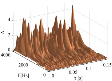
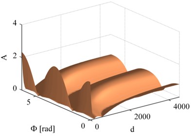
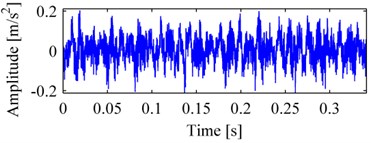
This is a problem of solving the maximum value, in order to choose the suitable atom, the inner product of each atom and residual should be calculated and compared with each other, and it usually needs many iterations before up to the termination condition, resulting in a large amount of computation. Reference [4] has proved that, when the length of the signal is fixed, with the increase of iteration steps, the residual decays exponentially, therefore, . Fig. 1 is the measured vibration signal of bearing with outer race fault, Fig. 2a, b displayed the functional diagram of inner product varied with the parameter group , obviously, this function is a complex multimodal function.
Fig. 1The vibration signal of bearing with outer race fault
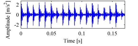
Fig. 2The diagram of the function of inner product: a) the function varies with τ and f, where ∅ and d are fixed, b) the function varies with ∅ and d, where τ and f are fixed
a)
b)
Therefore, the decomposition of vibration signals of bearings by MP_PA is solving the maximum value of a non-linear, non-differentiable, continuous and complex multimodal function, which cannot be directly solved by the techniques depending on gradient [9]. In order to meet the practical application, artificial intelligent algorithms were usually chosen to simplify the process of MP_PA, for example, genetic algorithm (GA) [6].
Only accurate extraction of features from signals especially for weak fault signals, the correct diagnosis could be achieved. NPSO which has received much attention in recent years could maintain good biodiversity and reduce the probability of falling into local optimal solutions, and it performs excellently for this kind of complex multimodal function [11, 13, 14].
2.2. The simplification of MP_PA by NPSO and SJ
2.2.1. The implement of MP_PA by NPSO
The implement of MP_PA by NPSO is simple, namely, in each iteration of MP_PA, the atom which satisfies is selected by NPSO, here is the iteration number of MP, and is the residual signal. In NPSO, the position of particle is , the fitness function is , after searching by particles, the position of the particle with the maximum fitness will be the parameter group which we are solving, i.e., the desired atom is obtained.
On the foundation of the features of MP_PA, the optimization in this paper was conducted by FERPSO (Fitness Euclidean-distance ratio PSO, a kind of NPSO) [11] and local optimization [13] and their excellent performance has been proved in reference [13]. The following briefly describes their improvements relative to PSO, the detailed explanation for this optimization procedure can be referred to [11, 13].
FERPSO is an effective local-best niching PSO which converges quickly and adopts fitness Euclidean-distance ratio (FER) value as an evaluation index, the difference from PSO is the velocity update mode of the particles, FERPSO uses a local optimum position which is determined by the largest FER value, instead of the global optimum position in velocity update equation. The FER value of particle corresponding to particle is determined by the relationship of their personal best positions previously visited, FER value is calculated using the following equation:
where is a scaling factor, is the Euclidian norm of the distance between the upper and lower of the search space, is fitness function. is the fittest particle in the current population, whereas is the worst fit particle; and are the current personal best positions of particle and particle , respectively. In FERPSO, the velocity update equation of each dimension for particle is modified as:
where all the symbols are the same as that in PSO except . represents the current evolution generation count, is the velocity of particle , is the inertia weight, and are both acceleration constants, and are two random numbers from a uniform distribution within the range of [0, 1], is the current position of particle , is the personal best position of the particle whose FER value is the largest with particle .
In order to further improve the performance of FERPSO, local optimization is added after the update of the velocity of particles, which not only enhances the fine-searching ability of the original niching PSO algorithms but also speeds up the convergence. The local optimization technique is to move a small step to or away the nearest personal best position of another particle (), the process is as follows:
Step 1, find ;
Step 2, if ,
let ;
otherwise, let .
Step 3, if , let .
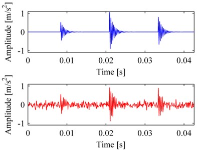
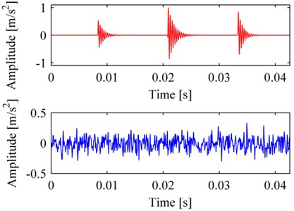
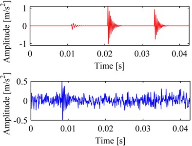
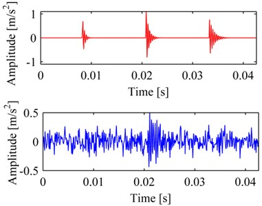
To test the performance of MP_PA which is implemented by FERPSO with local optimization, a simulated vibration signal of a bearing with defect was decomposed. In FERPSO, the number of the particles in the population was 30; the max iteration number was 300. The signal is a simulated vibration signal of a bearing with localized defects; it consists of a pulse sequence (as Eq. (5)) and Gaussian noise with signal to noise ratio (SNR) of 1dB. These signals are showed in Fig. 3a, it shows that the left pulse of signal is almost completely submerged in noise. After iterating three times of MP_PA using FERPSO, the results are illustrated in Fig. 3b, a comparison is also made by PSO and GA respectively in Fig. 3c, d. The comparison shows that MP_PA using FERPSO extracted the pulse components very well, and the SNR is as high as to 19 dB between the reconstructed signal and signal , and the SNR are 9 dB and 8 dB by PSO and GA, respectively. What’s more, we also test the three methods when the signal was added Gaussian noise with different SNR, and the results, which represent the average values from ten-time calculations, are listed as in Table 1, they furthermore indicate that FERPSO performs better when solving this problem.
where is a normalized pulse atom, the sampling frequency 12000 Hz.
Fig. 3The original signal and its decompositions: a) the simulated signal x' and signal x; reconstruction and residual by MP_PA simplified by different methods: b) FERPSO, c) PSO, d) GA
a)
b)
c)
d)
Table 1The results by FERPSO, PSO, GA with different noises
The SNR of noise | The SNR of the reconstruction by different methods | ||
FERPSO | PSO | GA | |
-3.0 dB | 13.2 dB | 7.1 dB | 5.3 dB |
-1.0 dB | 15.5 dB | 8.3 dB | 6.6 dB |
1.0 dB | 18.8 dB | 9.2 dB | 8.2 dB |
3.0 dB | 19.3 dB | 12.9 dB | 9.7 dB |
5.0 dB | 20.7 dB | 15.8 dB | 10.5 dB |
2.2.2. The simplification of MP_PA by SJ
When applying MP_PA to decompose a signal directly without the help of artificial intelligence algorithms, the selection of one suitable atom needs the computation complexity as follow:
where represents the computation of calculating one time the inner product of two signals whose length are both . With the same accuracy, if the signal’s length grows to , and the computation complexity will be:
Obviously, the amount of computation of is double to that of , and the amount of computation of is four times to that of . If the signal whose length is is divided into two signals whose length are both , because the total number of the selected atoms are the same, and then the computation complexity would reduce to one half. It means that decomposing a signal after segmentation will reduce the amount of computation, and the more the segments it has the less computation that needs. For example, if a signal is divided into eight segments with the same length, the computation complex will reduce to 1/8 of the origin. The experimental results in reference [10] show that, even if applying genetic algorithm, such kind of artificial intelligence algorithms to implement MP_PA, almost the same ratio of computation complexity will also be reduced due to segmentation.
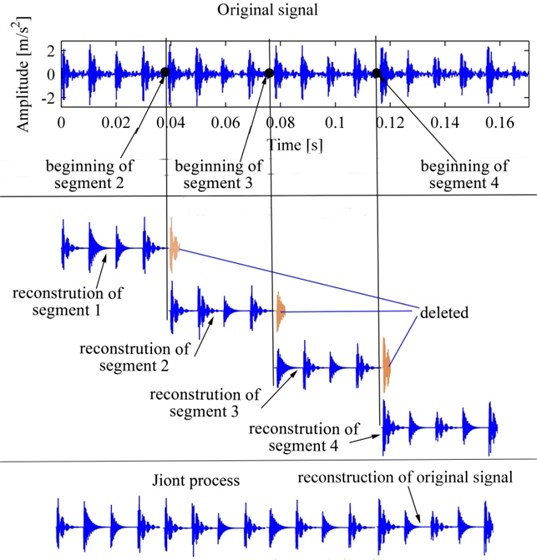
However, the fixed length of segmentation of original signal may divide the pulse components which locates at the endpoint of segments into two parts, this may cause error even wrong in process of decomposition (namely reconstruction), so an appropriate segmentation is necessary [17]. There are several segmentation techniques which have been introduced and successfully applied in different areas, such as an improved algebraic segmentation technique [17], the Kramers-Moyal coefficient method [18], statistical methods [19] and so on. In this paper, a simple and reasonable technique is employed, as shown in Fig. 4, let the segments overlap one by one, and make the overlap contain the pulse of the former segment, in joint process the overlap in the former segment will be deleted. The core of this technique is that the pulse which locates at the endpoint of a segment will be decomposed in next segment, and the beginning of one segment was selected adaptively according to the former one. The process is as follows: first, a proper fixed length of segments should be determined; here we let the duration of a segment be about one rotation of the bearing. Firstly, segment 1 is selected and decomposed (namely reconstructed), and then from the end of its reconstruction to forward, we find the point whose amplitude is less than a certain prespecified threshold which is near zero, then delete the part behind the selected point in its reconstruction, and make the point correspond to the selected point in original signal be the beginning of segment 2. Afterwards we decompose next segment one by one, until the whole signal is reconstructed, at last, all the reconstructions of segments are joined together one by one.
Fig. 4The process of SJ, the original signal is the same as Fig. 1
2.3. The multi features extraction based on parameters of pulse atom
2.3.1. The extraction of characteristic defect frequency based on DCS
It has been proved by Antoni [15], owing to the slight random slip between the rolling element and the cage, the pulse response induced by localized fault is not the same as the process of faulty gears which is of a purely periodic process, but close to second-order cyclostationary process. In the spectral correlation density of a failure bearing, the characteristic defect frequency displays as a prominent peak.
The methods based on cyclostationarity could eliminate the interference of random noises and improve the SNR, they have received more and more attentions in the application of the bearing fault diagnosis [15, 16, 20, 21]. As an important second-order cyclic statistic, DCS is defined on the foundation of cyclic autocorrelation function (CAF) or cyclic spectrum density (CSD) as follows:
where is the CAF, is cyclic frequency, is delayed time, is the CSD. It is known that DCS indicates the ratio of the energy of cyclic frequency to the energy of stationary part in the signal; DCS is a physical quantity which is able to completely describe the cyclostationarity. DCS is a function with cyclic frequency as the single variable, thus it is simpler than CAF or CSD which is a function of two variables. In theory, only if the signal is cyclostationary at the cyclic frequency , it will be that , otherwise , in actual fact, measured signal is complicated so that DCS is greater than 0 at many cyclic frequencies, in order to recognize the cyclic frequency clearly, the DCS is normalized in this paper.
After MP_PA, the conventional methods reconstructing signal accord to , but in this way it will also take the high resonance frequencies which are not help to extract characteristic defect frequency into the reconstruction. If we reconstruct signal in accordance with Eq. (9), namely each pulse atom is simplified to a pulse which occurs at the delayed time and the pulse’s amplitude is the same as the amplitude of atom, it should be noted that the reconstruction in this way is termed as pulse sequence, because the reconstruction will filter the resonance components and only preserves the low frequency components, the DCS of pulse sequence will become more simple and easy to identify. What’s more, because the DCS is obtained on the foundation of matching pursuit and DCS, it is termed as MP_DCS in this paper.
Taking into account the calculation error in actual fact, if we directly use the amplitude of the characteristic defect frequency as the feature value, it will inevitably be inconsistent with the practice. Therefore, the weighted sum of the amplitude of the characteristic defect frequency and its neighbors is taken as the feature value, as follows:
where is weighted sum, is characteristic defect frequency, is amplitude, is weighted factor, and , is frequency interval which equals the frequency resolution of DCS, and represents the number of weighted points.
2.3.2. The extraction of additional multi features
Besides the feature of characteristic defect frequency in the vibration signal of bearing with localized defects, there are other features, for example, the pulse energy will be much more than that of normal bearings; the signal will be dominated by high frequency due to some modes of resonance; what’s more, compared with normal bearings, the damping coefficients of pulses in fault ones will also vary. The parameters of pulse atom have explicit physical significances and almost contain all the information of pulses. If the features are extracted directly from these parameters, not only the process is more direct and convenient, but also the multi fault features could be extracted from multi dimensions, therefore, the diagnosis and detection would be more reliable and accurate. Consequently, besides characteristic defect frequency, the pulse components’ mean energy, frequency center and mean damping coefficients were all taken as features for better diagnosis, the equations based on parameters of pulse atoms are as follows:
where is the mean energy of pulse atoms, is the amplitude of atom, is the number of atoms.
where is frequency center, is resonance frequency of the pulse atom.
where is mean damping coefficient, is the damping coefficient of pulse atom.
2.3.3. Fault classification based on SVM
SVM is a machine learning algorithm based on statistical learning theory and structure risk minimization [22], it converts the optimization problem to a convex quadratic programming problem, and overcomes the problems of neural network such as its structure is complex, it is easy to fall into local minima and over learning, and has weak generalization capacity. SVM also has excellent learning ability and adaptability for small samples, and has been widely used in fault diagnosis in recent years [9, 23].
SVM multi-class classifier is generally constructed by multiple SVM two-classifiers combining together [24], for instance, one-against-all algorithm, and one-against-one algorithm. For the pattern recognition of bearing failure, to determine whether the bearing is failure or not is the most important issue, the second is the judgment which kind of failure. Therefore, the one-against-all algorithm is selected in this paper.
3. Experiment and discussion
3.1. The comparison of MP_DCS with WT and EMD
In the following analysis we used the rolling bearing data from the website of Case Western Reserve University, the model of rolling bearing is SKF 6205, the sampling frequency of the data is 12 kHz, the shaft speed is 1772 r/min, i.e., the rotation frequency 29.5 Hz, and the characteristic defect frequency of outer race failure 105.8 Hz, the characteristic defect frequency of inner race failure 159.9 Hz, and that of rolling element failure 139.2 Hz. In order to verify the performance of these techniques proposed, the weak fault of bearings in early stage which is a challenge was selected, namely, we chose the signals with more interference which was collected by the sensor placed on the base plate, the fault diameters was only 0.178 mm, and the load on bearing was just 1 horsepower. It should be noted that, because the data for normal bearing collected on the base plate is missing in the database, we used the data of normal status directly collected on the drive end instead, other test conditions are the same as mentioned above.
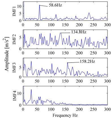
The length of the signals is 4096 points, and the length of each segment is 512 points. Because the atoms of low frequency do not satisfy the nature of pulse oscillating in high frequency, and they usually are trends and do not contain rich information about machine condition, only the atoms whose resonance frequency is above 300 Hz were selected when pulse sequence were reconstructed. At the same time, a comparison of wavelet envelope spectrum (WES) and EMD envelope spectrum (EMDES) of the raw vibration signals was also made, and the db8 wavelet was chosen as the basis wavelet. Pulse components tend to distribute in anterior intrinsic mode function (IMF) components [25], so that only the first four IMF components were displayed.
3.1.1. The analysis of normal bearing
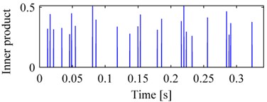
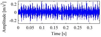
Fig. 5a is the vibration signal of normal bearing, we cannot determine which state the bearing is from Fig. 5a. Fig. 5b is the pulse sequence correspondingly, due to the high frequency interferences eliminated, only the pulses were reserved, as a result the pulse sequence is very sparse and easy to be calculated.
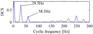
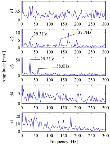
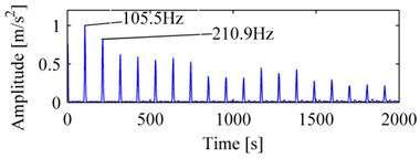
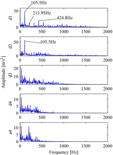
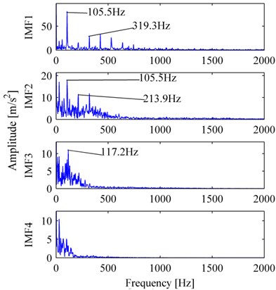
Fig. 5c is MP_DCS, the rotation frequency and its double could be seen clearly, and the amplitudes of the other frequencies are all very small, we could easily determine that the bearing is normal. Fig. 6a is WES corresponding to Fig. 5a, d1 to d4 are the envelope spectrum of the first to fourth levels of wavelet high frequency coefficients, a4 is the envelope spectrum of wavelet low frequency coefficient, the rotation frequency and its double could be seen in d2, d3 with many interference and including a peak of characteristic defect frequency of rolling element failure, it is difficult to determine the bearing condition and may cause confusion in a routine diagnostic survey. Fig. 6b is EMDES correspondingly, the rotation frequency or its double could be clearly identified only in IMF1, IMF2, however, there exists many interferential components resulting in difficult to diagnose.
Fig. 5The vibration signal of normal bearing and its decomposition: a) vibration signal of normal bearing, b) the pulse sequence, c) the DCS of pulse sequence
a)
b)
c)
Fig. 6The decomposition corresponding to Fig. 5(a): a) WES, b) EMDES
a)
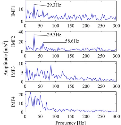
b)
3.1.2. The analysis of outer race failure bearing
Fig. 7a is the vibration signal of outer race failure, Fig. 7b, Fig. 8a, b are MP_DCS, WES and EMDES respectively of the fault signal. The outer characteristic defect frequency and its harmonics (up to eighteenth harmonic) are all clear and with few noises, these features indicate clearly that the bearing carries an outer race defect. In contrast, although the outer characteristic defect frequency and its harmonics could be recognized in WES or EMDES, they provide less explicit information about the condition of bearing, in addition, the random noise in the spectrum also blurs the featured components.
Fig. 7The vibration signal of the bearing with outer race failure and its MP_DCS: a) vibration signal of outer race, b) MP_DCS
a)
b)
Fig. 8The decomposition corresponding to Fig. 7(a): a) WES, b) EMDES
a)
b)
3.1.3. The analysis of inner race failure bearing
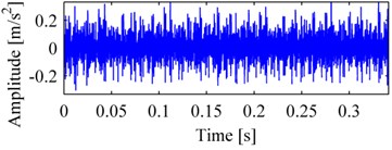
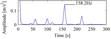
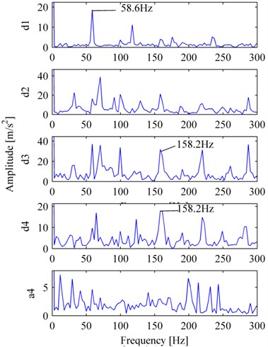
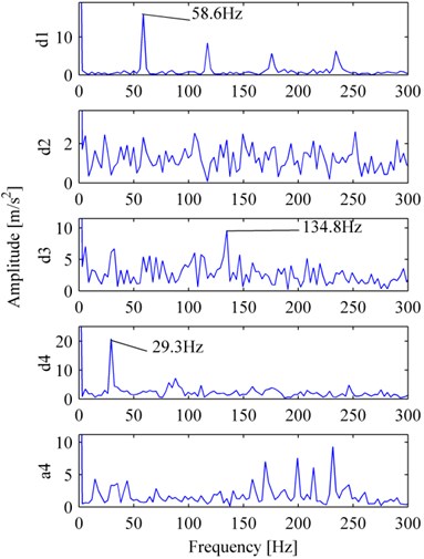
The inner race fault vibration signal is shown in Fig. 9a. Fig. 9b, and Fig. 10a, b are its MP_DCS, WES, and EMDES respectively. In Fig. 9b, the frequency of the peak with the largest amplitude is 158.2 Hz, is approximately the inner race characteristic defect frequency, hence we could determine that the bearing was failure in inner race. For WES, nevertheless there exist peaks of 158.2 Hz in d3 and d4, the amplitude of other frequencies, for example, 58.6 Hz (double of rotation frequency), are relatively high, thus it is a challenge to determine the bearing condition, a similar situation also occurs in EMDES.
Fig. 9The vibration signal of the bearing with inner race failure and its MP_DCS: a) vibration signal of outer race, b) MP_DCS
a)
b)
Fig. 10The decomposition corresponding to Fig. 9(a): a) WES, b) EMDES
a)
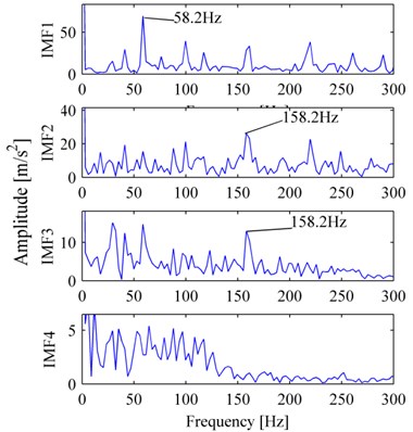
b)
3.1.4. The analysis of ball failure bearing
The ball fault vibration signal is shown in Fig. 11(a). Fig. 11(b), and Fig. 12(a), (b) are its MP_DCS, WES, EMDES respectively. In Fig. 11(b), from the peak with the frequency of 137.7 Hz, we can speculate that the bearing was ball failure. For WES, despite there exists ball characteristic defect frequency in d3, but the peak is not prominent enough, and it has been almost submerged in interferential components. For EMDES, it displays as a peak of ball characteristic defect frequency, as well as the inner race characteristic defect frequency, on the other hand it produces more irrelevant components which do not contribute to fault features and can further lead to inaccurate diagnosis.
Fig. 11The vibration signal of the bearing with ball failure and its MP_DCS: a) vibration signal of outer race, b) MP_DCS
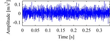
a)
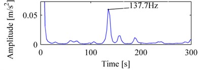
b)
Fig. 12The decomposition corresponding to Fig. 11(a): a) WES, b) EMDES
a)
b)
3.2. The analysis of multi features bearing diagnosis
From the comparison above, we can know that MP_DCS combines the advantages of matching pursuit, pulse atoms and cyclostationary, it adaptively matches the pulse components with sparse and accurate representation, removes high-frequency noise and improves the SNR thereby accentuating the defect frequency components and conducting the identification with confidence. Whereas the methods of wavelet transform and EMD, not only need the appropriate selection of component of decompositions, but also exist many interferential components and noises in their spectra, these will play a bad role in the fault diagnosis of bearings.
Besides the characteristic defect frequency, MP_PA can extract other features easily, such as the mean energy, frequency center, mean damping coefficient, and an analysis will be illustrated in below.
Fig. 13The distribution of multi features of the bearings in different conditions
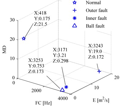
For accurate comparison, the signals should be collected in the same condition, thus we selected the signals collected by the sensor placed on the drive end, namely the same measured condition as the signal of Fig. 5a. After the raw signals were decomposed by MP_PA, the mean energy, frequency center, mean damping coefficient of the pulse atoms were calculated according to Eq. (11), (12), (13), respectively. Fig. 13 shows the results of bearings of different status, the multi features of fault bearings are greatly different from those of normal ones, the frequency centers of fault ones are much more than that of normal ones, as the same as the mean energy, these phenomena are consistent with failure mechanism.
3.3. The intelligent fault diagnosis of bearings based on SVM
In the following the extraction of multi features based on MP_PA and DCS was tested on an experimental measurement. The experiment equipment is shown in Fig. 14, the model of the bearings is HRB 6304, the sensor is B&K accelerometer, single point faults were created to the test bearings using electro-discharge machining with fault diameters of 0.53 mm and depth of 2.1 mm.
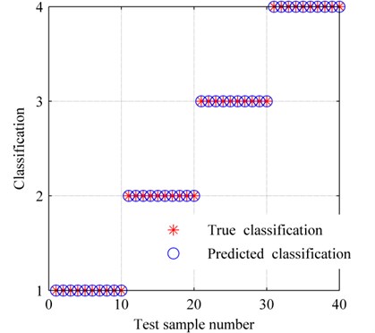
Firstly, each of 20 samples of data from normal state, outer race failure, inner race failure and ball failure bearings, namely a total of 80 sets of sample data were input to SVM learning machine, and then using this learning machine to predict the state of bearings in different status, the results are shown in Fig. 15, the accurate rate is as high as 100 %, it demonstrated that the multi-features-diagnosis based on MP_PA and DCS was effective and accurate, and meets the requirements for fault diagnosis of bearings.
Fig. 14The test rig
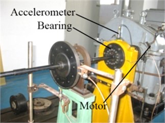
Fig. 15The SVM classification result, classification ‘1’ represents normal condition, ‘2’ is outer race fault, ‘3’ is inner race fault, and ‘4’ is ball fault
4. Conclusions
This paper employed simplified MP_PA based on the model of fault bearings and NPSO to obtain the parameters of atoms, on the foundation of these parameters and DCS we could acquire multi features, and identify the state of bearing effectively. The results showed that, this scheme has a simple and direct process, the features are prominent and the results are accurate, we could mainly come to these conclusions as follows:
(1) Firstly, from the model of fault bearings we derived the pulse atom, afterwards we explained that MP_PA was suitable for the bearing fault diagnosis in theory, and make the pulse atom parameters correspond with the fault features.
(2) The decomposition of vibration signals is equivalent to solving the maximum value of the high dimension and multimodal function, whose computation is considerably huge, and it is easy to be trapped into local optimal solutions by traditional artificial intelligent algorithms. To solve this problem, NPSO which is appropriate to this kind of problems was introduced, combined with SJ techniques to further reduce the amount of computation, at the same time the effectiveness of NPSO are verified by a simulated bearing fault signal.
(3) The periodicity of the pulse resonance sequence is not pure, but it have second-order cyclostationarity, consequently it is a good way to analyze the DCS of the pulse sequence which only preserve the low frequency components, and a comparison with WES and EMDES of the original signals were also made. The results showed that, MP_DCS could adaptively match the pulse components, has fine resolution and robust anti-interference ability, and provide more flexibility and accuracy for representing the vibration characteristics of rolling bearings.
(4) The multi features including the amplitude of characteristic frequency, mean energy, frequency center, mean damping coefficient, were applied to identify the status of the bearings based SVM, the accuracy rate was as high as 100 %, which means that these features can comprehensively reflect the condition of the bearings and are characterized by higher reliability.
References
-
Prashad H., Ghosh M., Biswas S. Diagnostic monitoring of rolling-element bearings by high-frequency resonance technique. ASLE Transactions, Vol. 28, Issue 4, 1985, p. 439-448.
-
Randall R. B., Antoni J. Rolling element bearing diagnostics – a tutorial. Mechanical Systems and Signal Processing, Vol. 25, Issue 2, 2011, p. 485-520.
-
Junsheng C., Dejie Y., Yu Y. Application of an impulse response wavelet to fault diagnosis of rolling bearings. Mechanical Systems and Signal Processing, Vol. 21, Issue 2, 2007, p. 920-929.
-
Mallat S. G., Zhang Z. Matching pursuits with time-frequency dictionaries. IEEE Transactions on Signal Processing, Vol. 41, Issue 12, 1993, p. 3397-3415.
-
Liu B., Ling S., Gribonval R. Bearing failure detection using matching pursuit. NDT & E International, Vol. 35, Issue 4, 2002, p. 255-262.
-
Stefanoiu D., Ionescu F. Faults diagnosis through genetic matching pursuit. Knowledge-Based Intelligent Information and Engineering Systems, Springer Berlin Heidelberg, 2003, p. 733-740.
-
Feng Z., Chu F. Application of atomic decomposition to gear damage detection. Journal of Sound and Vibration, Vol. 302, Issue 1, 2007, p. 138-151.
-
Goodwin M. Matching pursuit with damped sinusoids. 1997 IEEE International Conference on Acoustics, Speech, and Signal Processing, Vol. 3, 1997, p. 2037-2040.
-
Qin Q., Jiang Z. N., Feng K., He W. A novel scheme for fault detection of reciprocating compressor valves based on basis pursuit, wave matching and support vector machine. Measurement, Vol. 45, Issue 5, 2012, p. 897-908.
-
Cui L., Kang C., Wang H., Chen P. Application of composite dictionary multi-atom matching in gear fault diagnosis. Sensors, Vol. 11, Issue 6, 2011, p. 5981-6002.
-
Li X. A multimodal particle swarm optimizer based on fitness Euclidean-distance ratio. Proceedings of the 9th Annual Conference on Genetic and Evolutionary Computation, 2007, p. 78-85.
-
Engelbrecht A. P., Masiye B. S., Pampard G. Niching ability of basic particle swarm optimization algorithms. Swarm Intelligence Symposium, 2005, p. 397-400.
-
Qu B., Liang J., Suganthan P. Niching particle swarm optimization with local search for multi-modal optimization. Information Sciences, Vol. 197, 2012, p. 131-143.
-
Brits R., Engelbrecht A. P., Van Den Bergh F. A niching particle swarm optimizer. Proceedings of the 4th Asia-Pacific Conference on Simulated Evolution and Learning, Vol. 2, 2002, p. 692-696.
-
Antoni J., Randall R. Differential diagnosis of gear and bearing faults. Journal of Vibration and Acoustics, Vol. 124, Issue 2, 2002, p. 165-171.
-
Antoni J. Cyclostationarity by examples. Mechanical Systems and Signal Processing, Vol. 23, Issue 4, 2009, p. 987-1036.
-
Palivonaite R., Lukoseviciute K., Ragulskis M. Algebraic segmentation of short nonstationary time series based on evolutionary prediction algorithms. Neurocomputing, 2013.
-
Anteneodo C., Queirós S. M. D. Low-sampling-rate Kramers-Moyal coefficients. Physical Review E, Vol. 82, Issue 4, 2010, p. 041122.
-
Berkes I., Gabrys R., Horváth L., Kokoszka P. Detecting changes in the mean of functional observations. Journal of the Royal Statistical Society: Series B (Statistical Methodology), Vol. 71, Issue 5, 2009, p. 927-946.
-
McCormick A., Nandi A. Cyclostationarity in rotating machine vibrations. Mechanical Systems and Signal Processing, Vol. 12, Issue 2, 1998, p. 225-242.
-
Antoni J., Bonnardot F., Raad A., El Badaoui M. Cyclostationary modelling of rotating machine vibration signals. Mechanical Systems and Signal Processing, Vol. 18, Issue 6, 2004, p. 1285-1314.
-
Vapnik V. Statistical Learning Theory. Wiley, New York, 1998.
-
Yang Y., Yu D., Cheng J. A fault diagnosis approach for roller bearing based on IMF envelope spectrum and SVM. Measurement, Vol. 40, Issue 9, 2007, p. 943-950.
-
Thissen U., Van Brakel R., De Weijer A., Melssen W., Buydens L. Using support vector machines for time series prediction. Chemometrics and Intelligent Laboratory Systems, Vol. 69, Issue 1, 2003, p. 35-49.
-
Guo W., Tse P. W. A novel signal compression method based on optimal ensemble empirical mode decomposition for bearing vibration signals. Journal of Sound and Vibration, Vol. 332, Issue 2, 2013, p. 423-441.
About this article

