Abstract
Tool condition monitoring (TCM) takes an important position in CNC manufacturing processes, especially in damages avoiding of working parts and CNC itself. This paper presents a self-adaptive alarm method using probability density functions estimated with the Parzen window based on current signals, which gives an adaptively and rapidly corresponding alarm when the cutting tool fracture occurs. A CNC with cutting tools was obtained by Guangzhou CNC Company for test purpose, and the relative experiments were done in the state key laboratory. Current signals of the spindle motor and the main feed motor were acquired during the tool life. A probability model estimated with the Parzen window is established for current data fusion to alarm adaptively. At the meantime, the acoustic emission (AE) signals were acquired for comparison purpose. Experimental results show that this technique is flexible and fast enough to be implemented in real time for online tool condition monitoring.
1. Introduction
Tool condition monitoring plays an important role in modern automatic processing for ensuring the processing quality and the machine life [1-3]. It is important to study the abnormal state and alarm for tool condition monitoring. There are mainly two traditional tool monitoring alarm methods [4]: limit alarm and trend alarm. Limit alarm is that alarm when it is beyond the threshold which is defined statistically by experiences; trend alarm is that decides whether the faults occurred or will occur by the gradient change of monitoring parameters. As research progresses, many techniques and methods such as Fuzzy Logic (FL) [5], Neural Network (NN) [6] and Support Vector Machine (SVM) [7] have been used for monitoring alarm. They all obtained some effect on improving alarm intelligence and the adaptability of alarm threshold. While such techniques do have following disadvantages [8]: (1) working conditions and monitoring parameters cannot be adjusted dynamically by the fixed threshold, (2) the tool operating condition cannot be entirely reflected by the alarm algorithms.
In order to monitor the tool condition and alarm as early as possible, many researchers have investigated different sensors like accelerometer, acoustic emission transducer, current transducer and force sensor [9-11]. Since the current transducer is non-destructive evaluation, easily installed, non-effective on the normal operation of machine tool, and whose current signals has lower SNR (Signal Noise Ratio) [12], it has been selected for tool condition monitoring throughout this paper.
Research has shown that there exists a good linear relation between the spindle current and the tool wear [13]. The spindle current increases obviously when the cutting tool wears seriously or fails. On the other hand, cutting force is the direct reflection of tool condition, but the force sensor is hard to be installed. However, the change of cutting force leads to the change of the feed current. In general, the spindle current has simple frequency components and is influenced by operating condition greatly, while the feed current has complicated frequency components and is influenced by operating condition slightly. Therefore, the complementary spindle current and feed current are selected in monitoring the tool condition in the present work.
In this study, the self-adaptive alarm method using probability density functions estimated with the Parzen window is proposed. Current signals of the spindle motor and the main feed motor of a CNC are acquired during the tool life. According to their respective features, the amplitude of the spindle current and the root mean square (RMS) of the feed current are extracted. After that, a probability model estimated with the Parzen window is established for current data fusion to alarm adaptively.
2. The probability model estimated with the Parzen window
The Parzen window approach is widely used as a method in probability density estimation. It works properly in small samples and has smooth estimated curve. The Parzen window approach to obtain a non-parametric estimate from a collection of samples is applied as follows [14]. Consider the situation where we have a set of independent samples with an unknown underlying probability density function . Then the non-parametric estimate of from is provided by the function:
where is the window width coefficient, and is the sample dimension, and is a window or kernel function that integrates to unity. In the present work, by using Gaussian window, Eq. (1) is transformed to:
The Parzen window probability model is estimated by using the quantized values of the signals. Its physical interpretation has been shown in Fig. 1, in which the total probability density estimation is the sum of every sample’s Gaussian window.
Fig. 1Parzen window density estimation
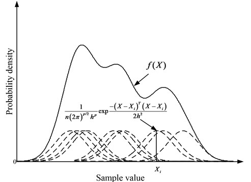
By Eq. (2), the shape of Gaussian window is mainly decided by . It becomes smoother as increases, while some details of the density function are buried. When is small, some details are described enough but the curve can be easily disturbed by random disturbance. Therefore, a proper is required to balance the above effects. In the present work, is calculated by:
where is an experience constant in [1.1, 1.4], and is the mean minimum distance between samples, given by:
3. Comprehensive alarm method for condition monitoring
3.1. Alarm boundary
When the machine is in a steady state, the monitoring data is large and the probability density function appears to be normal distribution approximately, where is the mean value and is the variance. Due to the 3 sigma rules, the probability that the monitoring parameters are in the range is 99.7 %. Therefore, is taken as the upper limit of the alarm in the present work.
As shown in Fig. 1, the probability density curve is close to the real distribution and therefore the boundaries are able to describe the monitoring parameters accurately. With the confidence level , the boundaries of satisfy:
where , are the upper and the lower confidence limit respectively. However, , calculated by Eq. (5) costs heavy computation, which is not suitable for online calculation.
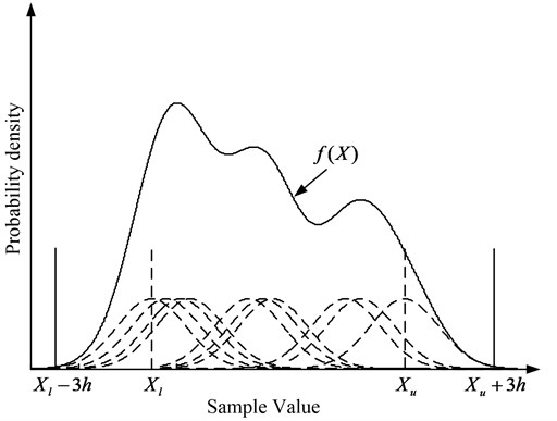
In the present work, Gaussian window is chosen in Eq. (2), therefore based on the traditional Pauta criterion, the density change caused by that is just 0.3 % [15], which can be ignored. Therefore, in the present work, we take the neighbourhood of monitoring parameters as the alarm threshold. The neighbourhood of the boundary samples is shown in Fig. 2, in which is the low boundary sample and is the upper boundary sample. is able to represent the low boundary of , and is able to represent the upper boundary of .
Fig. 23h neighbourhood of the boundary samples
Considering the two-dimensional monitoring parameters, taking every sample value as circle centre and as radius, the alarm boundary is formed by every circle. Due to the overlaps of circles, the alarm boundary is the envelope of all circles. Considering the high-dimensional monitoring parameters, the alarm boundary is a complex surface which is the envelope of all hyperspheres. The method to determine the alarm boundary is as shown in Fig. 3. After obtaining monitoring parameters, the mean minimum distance would be calculated, then followed by the window width coefficient and the Gaussian window function, we get the alarm boundary.
Fig. 3Method for determining alarm boundary
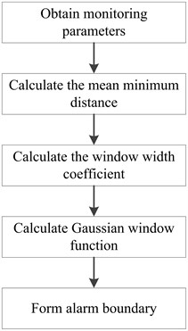
Fig. 4Comprehensive alarm method
3.2. Method of alarm
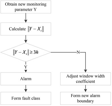
As the probability model is established by the data acquired in the normal operating condition, alarm occurs when the new monitoring parameter is beyond the alarm boundary. As shown in Fig. 4, the comprehensive alarm method is separated into two aspects based on the distance between the new parameter and the normal parameters. If the distance , alarm occurs and new fault classes would be built up. If , the window width coefficient would be adjusted and a new boundary would be formed.
3.3. Optimized method of alarm
Fig. 5Optimized algorithm for minimum distance
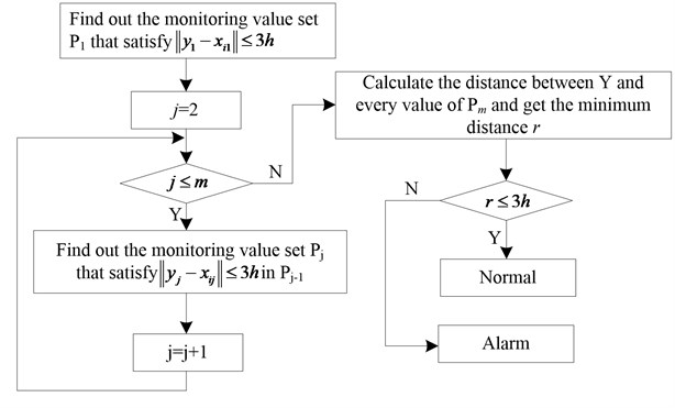
If the monitoring data is large, or high-dimensional, the calculation of the distance between new data and all existed data would be of low efficiency, which cannot meet the factual requirements. To improve this algorithm, we start by rapidly searching neighbouring points and cutting calculation times.
Suppose the monitoring parameter is a -dimensional vector, , the new monitoring value , then the optimized algorithm is as shown in Fig. 5.
By this method, we would achieve the shortest distance among data with few calculations to high-dimensional distance, and new monitoring data could be identified faster. Also, the probability density function would be updated as well, which forms a new alarm boundary. Further algorithm effect will be shown in the next section.
4. Simulations
A random 2-dimensional vector with length 65 and range [0, 1] was created by MATLAB. The original algorithm and the optimized algorithm are both applied to the vector. The results are shown in Fig. 6, in which the original boundary is composed of red “+”, and the optimized boundary is composed of black “o”. The calculation time is 23.81 s and 2.294 s respectively, which means that the calculation time of the optimized algorithm is reduced significantly.
Fig. 6The alarm boundaries of the original algorithm and the optimized algorithm
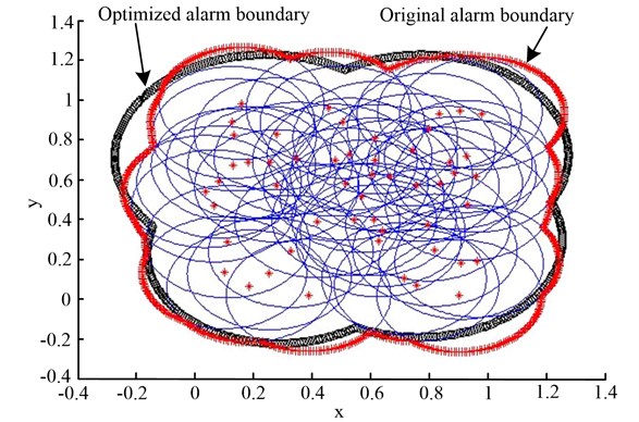
Fig. 7Running time of the original algorithm and the optimized algorithm
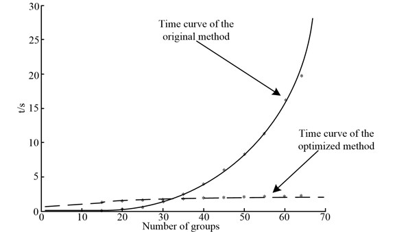
Furthermore, for the detail comparison of the calculation time, we select different data lengths that the original length is 15, 5 steps to the whole length 65. Then followed by the linear regression algorithm [16], the time curves are shown in Fig. 7. As shown in Fig. 7, the calculation time of the original algorithm is shorter when the data length is small, while as the length increases, the time increased sharply, but the time of the optimized algorithm increases smoothly. Therefore, the optimized algorithm is able to monitor tool condition with a high efficiency and precision for industrial requirements.
5. Experimental method
A CNC with cutting tools was studied by Guangzhou CNC Company. Tool life tests were carried out in the state key laboratory under a constant operating condition. The experimental setup is shown in Fig. 8 and the operating parameters are shown in Table 1. The current signals were acquired by two commercial current sensors (Fluke i200s). The sample rate is 2 kHz, and the sample time is 70 seconds per group. 60 groups of data were collected since the tool damage occurs at the 60th group.
Fig. 8Experimental setup

Table 1Operating parameters
Cutting tool | Rake angle | Relief angle | Work material | Spindle speed | Feed speed | Cutting depth |
Cemented carbide | 6º | 8º | Steel 45# | 800 rpm | 0.5 mm/m | 0.5 mm |
In above tests, an optical microscope (KEYENCE VHX-6000) with 1000x magnification was applied for observing the tool wear extent. Fig. 5 shows the wear extent in different stages.
Fig. 9Images during tool life

a) New tool

b) Initial wear

c) Fast wear

d) Stable wear

e) Stable wear

f) Stable wear

g) Sharp wear

h) Breakage
6. Signal processing and discussion
Fig. 10 depicts the current trends during the whole tool life. It can be seen that the characteristic values did not change much in the early stage since the tool is at the normal wear stage, while the value increases as the wear exacerbates. Also, the value increases sharply when the tool damage occurs.
Fig. 10Current trend through the tool life
a) RMS of feed current
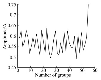
b) Amplitude of spindle current
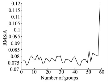
Due to the large differences of the characteristic values between the feed current and the spindle current, they are first normalized and then analysed by the optimized alarm method. Fig. 11 illustrates the result of the optimized alarm method. It shows that the alarm boundary is almost the envelope. As the new characteristic value is beyond the boundary at the 59th group, this method gives alarm, which means the tool wears seriously or fails and the machine should be stopped. Compared with Fig. 9, the result shown in Fig. 11 matches the fact and proves that this technique alarms adaptively under the occurrence of the cutting tool fracture and is able to meet the factual requirements.
For comparison, the AE signals were acquired at the meantime. Fig. 12(a) shows the raw AE signal at the time when the tool damage occurs, and its morphological filtered signal is shown in Fig. 12(b). Take the feature values of filtered signals as a 1-dimensional vector, and apply the optimized algorithm to the vector. The results are shown in Fig. 13, in which the historical curve is the trend of the feature values and the dynamic alarm curve is the boundary after optimized algorithm, and the detail view when the tool damage occurs is shown as well.
Fig. 11Result of the alarm method
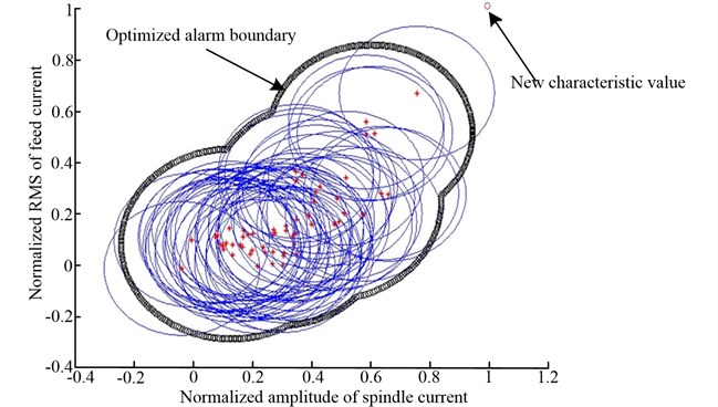
Fig. 12AE signals and feature extraction
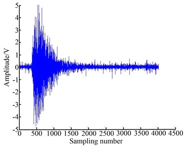
a) Raw AE signal
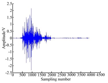
b) Morphological filtered signal
Fig. 13Alarm result based on AE signals
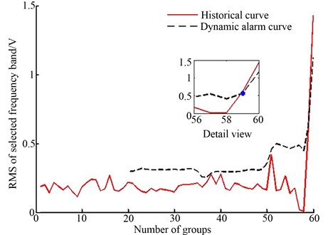
As shown in Fig. 13, at the 59th group, the feature value is below the alarm curve. The method based on AE signals gives alarm at the 60th group, while the method based on current signals gives alarm at the 59th group. This comparison proves the effectiveness and efficiency of the method based on current signals.
7. Conclusionss
In this paper, we proposed a self-adaptive alarm method for tool condition monitoring using probability density functions estimated with the Parzen window based on current signals by two steps. First, we calculated the window width coefficient with the help of the mean minimum distance between samples. Then it followed that the probability density function was estimated with the Parzen window and the alarm boundary had been formed. The data from current sensors were compared with those obtained from an AE transducer. The results were promising with the current signals. The main conclusions are as follows:
1. The non-contact current sensor could be considered as an attractive quality for tool condition monitoring.
2. Under data-accumulation, the window width coefficient and the alarm boundary are adjusted adaptively to make the alarm more accurate and adaptive.
3. The method based on current signals gives alarm earlier than the method based on AE signals.
4. The experimental result proves that this alarm method provides an adaptively and rapidly corresponding alarm when the cutting tool fracture occurs.
References
-
Dimla Sr. D. E., Lister P. M. On-line metal cutting tool condition monitoring. I: Force and vibration analyses. International Journal of Machine Tools and Manufacture, Vol. 40, Issue 5, 2000, p. 739-768.
-
Zhang L., Ji S. M., Xie Y., et al. Intelligent tool condition monitoring system based on rough sets and mathematical morphology. Applied Mechanics and Materials, Vol. 10-12, 2008, p. 61-65.
-
Roth J. T., Djurdjanovic D., Yang X., et al. Quality and inspection of machining operations: tool condition monitoring. Journal of Manufacturing Science and Engineering, Transactions of the ASME, Vol. 132, Issue 4, 2010, p. 0410151-04101516.
-
Liu G., Hao J., Kuang J. The machine plant accident alarm with trend and overage synthesis method. Journal of Agriculture University of Hebei, Vol. 23, Issue 4, 2000, p. 89-92.
-
Frank P. M. Residual evaluation for fault diagnosis based on adaptive fuzzy thresholds. IEE Colloquium (Digest), IEE Press, London, 1995, p. 1-11.
-
Zhang Q., Xu G. Incipient fault diagnosis based on moving probabilistic neural network. Journal of Xi’an Jiaotong University, Vol. 40, Issue 9, 2006, p. 1036-1040.
-
Zhang Q., Xu G., Hua C., et al. Self-adaptive alarm method for equipment condition based on one-class support vector machine. Journal of Xi’an Jiaotong University, Vol. 43, Issue 1, 2009, p. 61-65.
-
Massol O., Li X., Gouriveau R., et al. An exTS based neuro-fuzzy algorithm for prognostics and tool condition monitoring. International Conference on Control, Automation, Robotics and Vision, IEEE Computer Society, Piscataway, 2010, p. 1329-1334.
-
Chen X., Li B. Acoustic emission method for tool condition monitoring based on wavelet analysis. International Journal of Advanced Manufacturing Technology, Vol. 33, Issue 9-10, 2007, p. 968-976.
-
Heyns P. S. Tool condition monitoring using vibration measurements – A review. Insight: Non-Destructive Testing and Condition Monitoring, Vol. 49, Issue 8, 2004, p. 447-450.
-
Jemielniak K., Arrazola P. J. Application of AE and cutting force signals in tool condition monitoring in micro-milling. CIRP Journal of Manufacturing Science and Technology, Vol. 1, Issue 2, 2008, p. 97-102.
-
Guedidi S., Zouzou S. E., Laala W., et al. Induction motors broken rotor bars detection using MCSA and neural network: Experimental research. International Journal of Systems Assurance Engineering and Management, Vol. 4, Issue 2, 2013, p. 173-181.
-
Zhu K., Wong Y. S., Hong G. S. Wavelet analysis of sensor signals for tool condition monitoring: a review and some new results. International Journal of Machine Tools and Manufacture, Vol. 49, Issue 7-8, 2009, p. 537-553.
-
Rangaraj R. M., Wu Y. Screening of knee-joint vibroarthrographic signals using probability density functions estimated with Parzen windows. Biomedical Signal Processing and Control, Vol. 5, Issue 1, 2010, p. 53-58.
-
Krupinski R., Purczynski J. Approximated fast estimator for the shape parameter of generalized Gaussian distribution. Signal Processing, Vol. 86, Issue 2, 2010, p. 205-211.
-
Lai P. Y., Lee S. M. S. Estimation of central shapes of error distributions in linear regression problems. Annals of the Institute of Statistical Mathematics, Vol. 65, Issue 1, 2013, p. 105-124.
About this article

The authors gratefully wish to acknowledge the supports of the Major National Science and Technology Projects of P. R. China (Approval No. 2011ZX04016-031).
