Identification of piecewise linear aeroelastic systems

1. Introduction

Aeroelasticity is one of the prime concerns for an aircraft or a flight vehicle. The interaction of the aerodynamics and the structural dynamics of an aircraft could result in several different aeroelastic behaviors. These phenomena often exhibit nonlinear behaviors such as limit cycle oscillations (LCO), chaotic motions, coexisting stable solutions, bifurcations and so on [1-4]. Nonlinear factors in aeroelastic systems is ubiquity such as the material nonlinearity, the geometric nonlinearity, the freeplay nonlinearity and so on in structure, and the shock-boundary layer interaction, the flow separation, the unstable eddy current and so on in aerodynamics [5]. Freeplay nonlinearity can arise from worn hinges and loose attachments which are generally related with aircraft aging. The combination of freeplay nonlinearities with the aerodynamic and structural nonlinearities can vary the system’s response and change its instability from a supercritical to a subcritical one. These changes can result in catastrophic damages. To that end, many researchers have investigated numerically and experimentally the effects of freeplay nonlinearity on aeroelastic systems [6-10].

In order to study a nonlinear aeroelastic system with a freeplay nonlinearity, its accurate mathematics model needs to be constructed first. In engineering practice, freeplay such as gap in the bolt connection [9] may never be correctly measured, so the mathematic models of these systems have to be constructed by identification of experimental data. For example, the aeroelastic systems with freeplay can be identified by representing the freeplay as a polynomial [11] and a hyperbolic tangent function [12], respectively. It was pointed out that the locations of the switching points of the freeplay nonlinearity are of importance in the modeling process, which not only influence the location of bifurcation points, but also impact the dynamic behaviors [10]. Since the switching points in these identified models are eliminated artificially, their dynamic behaviors are different from the original systems in essence [11, 12]. Recently, a non-parameter method was developed to identify the switching points of freeplay [13]. But this method needs the bandwidth of the kernel function, and unfortunately the selection of the bandwidth depends strongly on the engineer experience and influences the precision of the switching points.

The objective of this work is to identify and construct the mathematic model of the nonlinear aeroelastic system with a freeplay nonlinearity. This is achieved and demonstrated by performing system identification of a two-dimensional airfoil with a freeplay nonlinearity in the pitch degree-of-freedom. The system model makes use of pitch–plunge governing equations with quasi-steady approximation of the aerodynamic loads.

2. The aeroelastic model

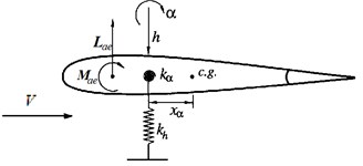
The model here is a two-dimensional airfoil with nonlinear structural freeplay in the pitch degree-of-freedom. A schematic of the airfoil section with a trailing-edge flap for control actuation [14] is shown in Fig. 1. This system, which has been studied extensively in the literature, can be modeled by a pair of coupled second-order differential equations [15]:

where $h$ denotes the plunge displacement of the airfoil and $\alpha$ represents the pitch angle. Other variables include the non-dimensional distance between the elastic axis and the center of mass $x_{\alpha }$, the mass of the wing $m$, the mass moment of inertia $I_{\alpha }$, semi-chord length $b$, structural damping coefficients in plunge and pitch $c_h$ and $c_{\alpha }$, and spring constants $k_h$ and $k_{\alpha }$. The lift $L_{ae}$ and moment $M_{ae}$ are determined by quasi-steady aerodynamic theory. The parameters $c_{l\alpha }$ and $c_{l\alpha }$ are introduced to represent the lift and moment coefficients for angle of attack, $c_{l\beta }$ and $c_{m\beta }$ are introduced to represent the lift and moment coefficients for control surface position, $a$ is the non-dimensional distance between the middle of the chord and the elastic axis, $\rho$ is density of air and $V$ is free stream velocity.

Fig. 1Airfoil model

a)

b)

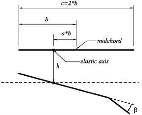
With a structural freeplay gap, the pitch-restoring moment-rotation relationships $M_{\alpha }\left(\alpha \right)$ are illustrated in Fig. 2 as:

where ${\delta }_1$ and ${\delta }_2$ are the switching points, $M_0$ is the restoring moment at the start of the freeplay and shown in Fig. 2.

Fig. 2Freeplay nonlinearity in the pitch direction model

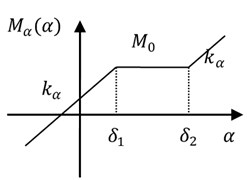
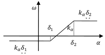
Fig. 3Saturation function ω

By substituting Eq. (2) and Eq. (3) into Eq. (1), the transformed equations of motions in the state space form become:

where $\mathit{X}={\left[\begin{array}{cc}\begin{array}{cc}h& \alpha \end{array}& \begin{array}{cc}\dot{h}& \dot{\alpha }\end{array}\end{array}\right]}^T$, $T$ denotes the matrix or vector transpose,

$\omega =f\left(\alpha \right)=k_{\alpha }\alpha -M_{\alpha }\left(\alpha \right)$, $\mathit{M}=\left[\begin{array}{cc}m& m{x}_{\alpha }b\\ m{x}_{\alpha }b& I_{\alpha }\end{array}\right]$, $\mathit{K}=\left[\begin{array}{cc}{k}_h& \rho V^{2}b{c}_{l\alpha }\\ 0& k_{\alpha }-\rho V^2{b}^2{c}_{m\alpha }\end{array}\right]$,

$\mathit{C}=\left[\begin{array}{cc}{c}_h+\rho Vb{c}_{l\alpha }& \rho V{b}^2{c}_{l\alpha }\left(0.5-a\right)\\ -\rho V{b}^2{c}_{m\alpha }& c_{\alpha }-\rho V{b}^3{c}_{m\alpha }\left(0.5-a\right)\end{array}\right]$, ${\mathit{F}}_1=\left[\begin{array}{c}-\rho V^{2}b{c}_{l\beta }\\ \rho V^2{b}^2{c}_{m\beta }\end{array}\right]$, ${\mathit{F}}_2=\left[\begin{array}{c}0\\ 1\end{array}\right]$,

$\mathit{A}=\left[\begin{array}{cc}0& \mathit{I}\\ -{\mathit{M}}^{-1}\mathit{K}& -{\mathit{M}}^{-1}\mathit{C}\end{array}\right]$, ${\mathit{B}}_1=\left[\begin{array}{c}0\\ {\mathit{M}}^{-1}{\mathit{F}}_1\end{array}\right]$, ${\mathit{B}}_2=\left[\begin{array}{c}0\\ {\mathit{M}}^{-1}{\mathit{F}}_2\end{array}\right]$, $\mathit{I}$ denotes the identity matrix.

The saturation function $\omega$ is illustrated in Fig. 3 as:

Substituting Eq. (6) into Eq. (5) as:

where ${\mathit{D}}_1={\mathit{B}}_2{k}_{\alpha }{\delta }_2$, ${\mathit{D}}_2={\mathit{B}}_2{k}_{\alpha }$, ${\mathit{D}}_3={\mathit{B}}_2{k}_{\alpha }{\delta }_1$, $\mathit{H}={\mathit{B}}_2{M}_0$.

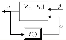
The airfoil model output is the pitch angle $\alpha$. Using a nonlinear feedback linear fractional transformation (LFT) [16], Eq. (5) represents as:

where $\mathit{P}$ is the nominal plant and:

where $P_{1k}\left(k=1,2\right)$ are the functions related to the input ${\left\{\beta ,\omega \right\}}^T$and output $\alpha$ signals. These transfer function matrices are built from the $\mathit{M}$, $\mathit{C}$, $\mathit{K}$, ${\mathit{F}}_1$ and ${\mathit{F}}_2$ matrices of the nominal aeroelastic model. $F_l\left[\bullet ,\bullet \right]$ denotes the low LFT. Eq. (8) is illustrated in Fig. 4 [16]. According to Eq. (5), $P_{11}$ and $P_{12}$ can be represented as:

where $\mathit{Q}=\left[\begin{array}{cc}\begin{array}{cc}0& 1\end{array}& \begin{array}{cc}0& 0\end{array}\end{array}\right]$ and $s$ is Laplace variable.

Fig. 4LFT with saturation function fα

According to LFT algebra, Eq. (8) can also be represented as:

where $P_{11}\beta$ is the linear part of the output $\alpha$, and $P_{12}f\left(\alpha \right)$ is the nonlinear part of the output $\alpha$ and a Hammerstein model, which comprises of a static nonlinearity followed by a linear time invariant system [16].

3. Identification of the poles of the linear subsystem

4. Identification of the switching points

Let us define ${\lambda }_k=P_{22}f\left({\alpha }_k\right)$, which is the nonlinear part of the output ${\alpha }_k$ in Eq. (11) and also a discrete Hammerstein model [16], which comprises of a saturation function $f\left(\bullet \right)$ followed by a linear time invariant system $P_{22}\left(q\right)$ connected, shown in Fig. 5.

Define a switching function $h\left(u\right)$as follows:

The saturation function$f\left(\bullet \right)$is:

where $g_1\left({\alpha }_{k-1},{\delta }_1,{\delta }_2\right)={\alpha }_{k-1}\left[h\left({\delta }_2-{\alpha }_{k-1}\right)-h\left({\delta }_1-{\alpha }_{k-1}\right)\right]$;

$g_2\left({\alpha }_{k-1},{\delta }_1,{\delta }_2\right)=h\left({\alpha }_{k-1}-{\delta }_2\right)$; $g_3\left({\alpha }_{k-1},{\delta }_1,{\delta }_2\right)=h\left({\delta }_1-{\alpha }_{k-1}\right)$; $g_4\left({\alpha }_{k-1},{\delta }_1,{\delta }_2\right)=-1$;

$d_1=k_{\alpha }$; $d_2=k_{\alpha }{\delta }_2$; $d_3=k_{\alpha }{\delta }_1$; $d_4=M_0$; the parameters $d_1$, $d_2$, $d_3$ and $d_4$ are unknown.

The linear system $P_{22}\left(q\right)$ in Eq. (14a-c) can be represented by using the orthonormal basis functions ${\left\{B_l\left(q\right)\right\}}_{l=0}^{p-1}$ [20] which are constructed by using the poles of linear part of the nonlinear system as follows:

where $P_{22}\left(q\right)\in \mathit{R}\left(\mathbb{Q}\right)$, $\mathbb{Q}$ is the unit circle [16] and the parameter $e_l\in R$ is unknown.

The input-output relationship of the system illustrated by Fig. 5 is:

where ${\lambda }_k$ and ${\eta }_k$ represent the system output and measurement noise at time $k$, respectively.

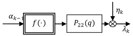
Fig. 5. Hammerstein model

The linear system $P_{21}\left(q\right)$ in Eq. (14)a-c) represents by using the orthonormal basis functions ${\left\{B_l\left(q\right)\right\}}_{l=0}^{p-1}$ [20] as follows:

When Eq. (21) and Eq. (22) are substituted into Eq. (14a-c), the input-output relationship can be written as:

Let’s now define:

When Eq. (24a) and Eq. (24b) are placed into Eq. (23), the later results in the regression vector:

Now, with the simulated data set ${\left\{{\beta }_k,{\alpha }_k\right\}}_{k=1}^N$ of the nonlinear aeroelastic system with freeplay and defining the matrices ${\mathit{X}}_N\triangleq {\left[{\alpha }_1,\cdots ,{\alpha }_N\right]}^T\text{,}$${\mathit{\Gamma }}_N\triangleq {\left[{\eta }_1,\cdots ,{\eta }_N\right]}^T$ and ${\mathit{\Phi }}_N\triangleq \left[{\mathit{\varphi }}_1,\cdots ,{\mathit{\varphi }}_N\right]$, we obtain:

First, the initial values of the switching points ${\delta }_1$ and ${\delta }_2$ are given and ${\mathit{\varphi }}_k$ is calculated. The estimated $\widehat{\mathit{\theta }}$ of the parameters $\mathit{\theta }$ are obtained by using the least square estimation or the bias-eliminated least square method [19]. According to the definition of the parameter $\mathit{\theta }$, its first $p$ parameters are the coefficients of the linear part $P_{21}\left(q\right)$, and the else are the coefficients of the nonlinear part $P_{22}\left(q\right)f\left(\bullet \right)$. Since the parameters of the saturation function$f\left(\bullet \right)$ and the linear system $P_{22}\left(q\right)$ are coupling, the unique estimated parameters $d_1\text{,}$$d_2\text{,}$$d_3\text{,}$$d_4$and $b_l$$\left(l=0,1,\cdots ,p-1\right)$ can be obtained if the parameter $\mathit{d}={\left[\begin{array}{cc}\begin{array}{cc}{d}_1& d_2\end{array}& \begin{array}{cc}{d}_3& d_4\end{array}\end{array}\right]}^T$ are normalized, that is, ${‖\mathit{d}‖}_2=1$ [16]. Since the parameters $\mathit{d}$ are normalized, the identified parameters $d_1$, $d_2$, $d_3$ and $d_4$ lose the physical significance defining in the above, but the switching points ${\delta }_1$ and ${\delta }_2$ can be estimated by ${\widehat{\delta }}_1={\widehat{d}}_3/{\widehat{d}}_1$ and ${\widehat{\delta }}_2={\widehat{d}}_2/{\widehat{d}}_1$. Using the renewed switching points ${\widehat{\delta }}_1$ and ${\widehat{\delta }}_2$ repeat the above identified procedure until the convergence of the switching points ${\delta }_1$ and ${\delta }_2$. Then all parameters of this nonlinear model including the switching points can be obtained.

5. A simulated example

The parameters of a two-dimensional airfoil with nonlinear structural freeplay in the pitch degree-of-freedom to be used in the numerical simulation are given in Table 1. The output of the simulated measured system is the pitch angle $\alpha \left(t\right)$, which is corrupted with additive Gaussian distributed white noise with a signal-to-noise ratio of 20 dB, and the input is the flap deflection $\beta \left(t\right)$, which is a zero-mean Gaussian distributed white noise with standard deviation 10. A key issue in the time marching integration of a piecewise linear system is accurately integrating to the “switching points” where the change in linear subdomains occurs. It is indicated that a standard time marching scheme, for example, the Runge-Kutta method with the uniform time step, may lead to inconsistent or even incorrect numerical results [21]. In this paper, the response of the system in the first 50 seconds is computed by using the Henon’s method [22, 23] whose time step is $t_s=\text{0.001 s}$.

It is easy to know the number of the degree-of-freedom for the discrete system. This sumulated model has two degree-of-freedoms. Assuming $A\left(q\right)$ and $B\left(q\right)$ are:

According to section 3.2, we may as well assume $h_1=$ 0.4 and $h_2=$ -0.1 since ${\tilde{\alpha }}_N=$ 0.7307 and ${\tilde{\alpha }}_1=$ -0.7454. Here selecting $h_1=$0.4 and $h_2=$ -0.1 make full of the input-output data in order to eliminate measurement noise. When $h_1=$ 0.4 is used, the parameter $\mathit{\mu }$ is estimated by the bias-eliminated least square method [19], and given in Table 2; when $h_2=$ -0.1 is used, the parameter$\mathit{}\mathit{\mu }$ is estimated by the bias-eliminated least square method [19], and also given in Table 2. The estimated parameters are the same in $h_1=$ 0.4 and $h_2=$ -0.1 cases except $r_1\ne r_3$. The parameter $r_1\ne r_3$ is caused by the asymmetric switching points of a freeplay nonlinearity.

According to the relationship of poles of the discrete system with the continue system $\gamma ={\mathrm{e}}^{t_s\kappa }$ ($\kappa$ and $\gamma$ denote a pole of the discrete system and the one of the corresponding continue system pole, respectively), the frequency $f_i$ and damping ${\zeta }_i$ ($i=1,2$) of these two physical modes of the linear part of the nonlinear airfoil are given in Table 3. In Table 3, the second column indicates the frequency and damping of the true modes. The third and fourth columns present the estimated frequency and damping of the true modes using the proposed method in section 3. Comparing the estimated modes and true modes in Table 3, it is obvious to see that the frequency $f_i$ and damping ${\zeta }_i$$\left(i=1,2\right)$ of these two physical modes are estimated consistently.

The poles of the linear part of the nonlinear model are the same with the ones of the first and third linear subsystem, that is Eq. (15a) and Eq. (15c). The poles and the orthonormal basis functions constructed by them [20] are:

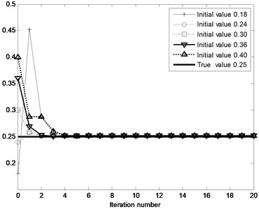
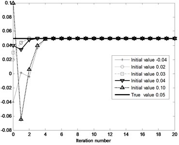
The convergence of the switching points ${\delta }_2$ and ${\delta }_1$ are illustrated in Fig. 6, when the initial switching points ${\delta }_2$ and ${\delta }_1$ are (0.18, -0.04), (0.24, 0.02), (0.30, 0.03), (0.36, 0.04) and (0.40, 0.10). It is found from Fig. 6 that the switching points are converged to the true values only through the 6 steps iteration, and meanwhile it is stated that the convergence of the switching points is good when the different initial value of the switching points ${\delta }_2$ and ${\delta }_1$ are utilized. When the initial value of the switching point ${\delta }_2$ and ${\delta }_1$ are (0.40, 0.10), through the 20 steps iteration the estimated parameters of the system are: ${\widehat{\tau }}_0=\text{7.4606×}{\text{10}}^{\text{-3}}\text{,}$${\widehat{\tau }}_1=\text{4.9613×}{\text{10}}^{\text{-3}}\text{,}$${\widehat{\tau }}_2=\text{-1.7787×}{\text{10}}^{\text{-2}}\text{,}$${\widehat{\tau }}_3=\text{-5.2651×}{\text{10}}^{\text{-3}}$, ${\widehat{d}}_1=\text{0.9642}$, ${\widehat{d}}_2=\text{0.2424}$, ${\widehat{d}}_3=\text{0.04806}$, ${\widehat{d}}_4=\text{0.09645}$, ${\widehat{e}}_0=\text{1.6616×}{\text{10}}^{\text{-2}}$, ${\widehat{e}}_1=\text{-1.5177×}{\text{10}}^{\text{-2}}\text{,}$${\widehat{e}}_2=\text{7.4796×}{\text{10}}^{\text{-2}}\text{,}$${\widehat{e}}_3=\text{1.6150×}{\text{10}}^{\text{-2}}$. The identified switching points are ${\widehat{\delta }}_2=\text{0.2514}$ and ${\widehat{\delta }}_1=\text{0.04985}$, and the true switching points are ${\delta }_2=\text{0.25}$ and ${\delta }_1=\text{0.05}$. The relative errors which are caused by the number computation are 0.5573 % and 0.3052 % and satisfied the engineering requirements.

Fig. 6Convergence of switching points δ2 and δ1: a) the initial values of switching point δ2 are 0.18, 0.24, 0.30, 0.36 and 0.4; the true value of switching point δ2 is 0.25, b) the initial values of switching point δ1 are -0.04, 0.02, 0.03, 0.04 and 0.10; the true value of switching point δ1 is 0.05

a)

b)

Fig. 7Output of nonlinear system (dotted line) and identified nonlinear model (solid line) with Gauss white noise input: a) with measurement noise, b) without measurement noise

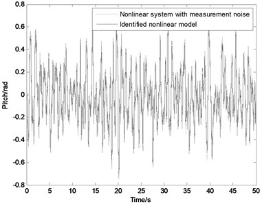
a)

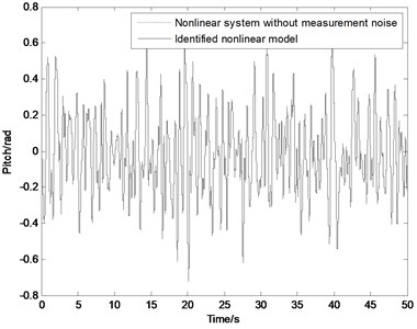
b)

Fig. 7 shows the output of the nonlinear system (dotted line) and the identified nonlinear model (solid line) with the Gauss white noise input. Because of the output of nonlinear system with the measurement noise in Fig. 7(a), there is a clear difference between them. In Fig. 7(b) they are almost coincided due to the outputs without the measurement noise. The validity of the identified nonlinear model is checked by several other input signals without shown here.

6. Conclusions

In this paper, a novel identification algorithm is proposed for the estimation of the nonlinear system with freeplay. In this algorithm, an orthonormal basis function expansion and a Hammerstein model are applied to represent the linear and nonlinear parts of the system, respectively; and an orthonormal basis function expansion and the constructional basis functions $g_i\left({\alpha }_{k-1},{\delta }_1,{\delta }_2\right)\left(i=1,2,\cdots ,4\right)$ are used to represent the linear and nonlinear functions of the Hammerstein model. An approach synthesized of the non-iterative and iterative algorithms is implemented to estimate the parameters of the system including the switching points. Furthermore, a method is proposed to estimate physical poles of the system which could be essentially reduced to a linear parametric problem by a simple data rearrangement in an ascending order according to their values. Thus, the data which is concerned with the degree-of-freedom of the freeplay nonlinearity are partitioned into three data sets that correspond to distinct linear regression models. Later on the estimates of unknown parameters of linear regression models can be calculated by processing respective sets of the rearranged input and associated output observations. The consistent estimation of these physical poles plays a crucial role for the generation of the orthonormal basis functions and for the model approximation results.