Simultaneous excitation and parameter identification for non-linear structural systems

2.1. Discrete-time state-space model of structural dynamics

The general equation of motion of a damped structure with $n$ DOFs can be written as:

where $\mathbf{M}\text{,}$$\mathbf{C}$ and $\mathbf{K}\in {\mathbb{R}}^{n\times n}$ are the mass, damping and stiffness matrices of the structure, respectively; $\ddot{\mathbf{p}}\left(t\right)$, $\dot{\mathbf{p}}\left(t\right)$, $\mathbf{p}\left(t\right)\in {\mathbb{R}}^n$ are, respectively, the nodal acceleration, velocity and displacement vectors of the structure; $\mathbf{u}\left(t\right)\in {\mathbb{R}}^m$ is the force vector and ${\mathbf{B}}_u\in {\mathbb{R}}^{n\times m}$ is the influence matrix associated with $\mathbf{u}\left(t\right)$.

The second-order equation of motion Eq. (1) can be transformed into a first-order continuous-time state equation as:

where $\mathbf{x}\left(t\right)\in {\mathbb{R}}^{2n\times 2n}$ is the state vector, and the system matrices together with $x\left(t\right)$ are defined as:

Assuming that only s acceleration signals are measured (i.e. $y\left(t\right)\in {\mathbb{R}}^s$), the measurement equation can be written as the following state-space form:

With the output influence matrix $\mathbf{H}\in {\mathbb{R}}^{s\times n}$ and direct transmission matrix $\mathbf{D}\in {\mathbb{R}}^{s\times m}$ defined as:

where the ${\mathbf{H}}_0$ is the selection matrix of appropriate dimension for accelerations and composed by zeros and ones.

Let the symbol $\mathrm{\Delta }t$ denote the time step size, thus the continuous-time state-space model of Eqs. (2) and (4) can be transformed into the following discrete-time form using a sampling rate of 1/$\mathrm{\Delta }t$:

where:

2.2. The GDF algorithm

Considering the system and measurement noise, the linear structural system can be rewritten as:

The system noise vector ${\mathbf{w}}_{\mathbf{k}}\in {\mathbb{R}}^n$ and measurement noise vector ${\mathbf{v}}_k\in {\mathbb{R}}^m$ are assumed to be mutually uncorrelated, zero-mean, white random signal with known covariance matrices, ${\mathbf{G}}_k=E\left\{{\mathbf{w}}_k{\mathbf{w}}_l^T\right\}$ and ${\mathbf{R}}_k=E\left\{{\mathbf{v}}_k{\mathbf{v}}_l^T\right\}$ respectively ($E$ represents the expectation value). Results are easily generalized to the case where ${\mathbf{w}}_{\mathbf{k}}$ and ${\mathbf{v}}_k$ are correlated [21]. If the inputs ${\mathbf{u}}_k$ in Eqs. (10) and (11) are unknown, then the two equations represent the linear dynamic system with direct feedthrough. In the field of system control, Gillijns and De Moor proposed an optimal recursive filter of the direct feedthrough case for joint input/state identification [20]. In this filter, a state estimate ${\mathbf{x}}_{k|l}$ is defined as an estimate of ${\mathbf{x}}_k$ given $\{{\mathbf{y}}_0,{\mathbf{y}}_1,\dots ,{\mathbf{y}}_l\}$ and its error covariance matrix ${\mathbf{P}}_{k|l}^x$ as $E\left[\right({\mathbf{x}}_k-{\mathbf{x}}_{k|l}\left)\right({\mathbf{x}}_k-{\mathbf{x}}_{k|l}{)}^T]$. An initial unbiased state estimate ${\mathbf{x}}_{0|-1}$ and its covariance matrix ${\mathbf{P}}_{0|-1}^x$ are assumed known.

The GDF algorithm computes the unknown input and state in a recursive procedure which includes three steps: the input identification, the measurement update and the time update. The GDF algorithm is listed in Table 1.

In Ref. [22], the GDF is applied in linear structural dynamics for joint input/response identification successfully. However, it is not suitable for non-linear dynamic systems. In Section 3, the GDF method is extended for non-linear dynamic system to solve the problem of coupled state/input/parameter identification.

3.1. Non-linear identification model of the coupled state/input/parameter identification

Assuming in dynamics Eq. (1) that only $\mathbf{K}$ and $\mathbf{C}$ contain the uncertain parameters $\alpha$ to be identified, the original state vector $\mathbf{x}$ can be extended to be the augmented state vector as:

where $\alpha =[\begin{array}{llll}{\alpha }_1& {\alpha }_2& \cdots & {\alpha }_{\alpha }\end{array}{]}^T\in {\mathbb{R}}^{\alpha }$ is the parameter vector. Therefore, the augmented state transmission and measurement equations can be obtained as:

The parameters are assumed to be constant, i.e. $\dot{\alpha }=\left[0\right]$.

The above continuous-time state-space equations can be transformed into the following form as:

Unlike Eqs. (10) and (11), the functions $f$ and $h$ are both non-linear. The standard GDF method cannot be adopted to handle this case of non-linear identification. In the research field of system control, the standard KF was presented for identifying the state of linear dynamic systems. The EKF algorithm was then developed for identifying the state of non-linear dynamic systems by continually updating a linearization around the previous state estimate, starting with an initial guess, which is a non-linear variation on the standard KF based on the first-order Taylor approximation. In the following section, the linearization idea of the EKF method is adopted to extend the standard GDF method for non-linear dynamic systems.

3.2. The extended GDF algorithm

In this coupled state/input/parameter identification problem, the augmented state ${\mathbf{z}}_k$ (including state and uncertain parameters) and identified forces ${\mathbf{u}}_k$ are both unknown. Therefore, we have the first-order Taylor series expansions for the two non-linear system matrices:

where ${\nabla }_z{f}_k$, ${\nabla }_u{f}_k$ and ${\nabla }_z{h}_k$ are the sensitivity matrices, and $HOT$ stands for the high-order terms.

Using the Taylor expansions, the Eqs. (17) and (18) can be approximated in the following linear form:

Then, the prior expectation of the augmented state vector ${\mathbf{z}}_k$ has the approximately linear form as:

Using the three approximately linear Eqs. (19)-(21), the proposed extended GDF (EGDF) algorithm can be derived referring to Ref. [20]. The EGDF algorithm is shown in Table 2. With the algorithm, the augmented state $\mathbf{z}$ and the excitation $\mathbf{u}$ can be simultaneously identified.

Comparing the EGDF algorithm with the standard GDF algorithm, it is found that the two algorithms are very similar, and the only differences are the three sensitivity matrices of ${\nabla }_{\mathbf{z}}{f}_k$, ${\nabla }_{\mathbf{u}}{f}_k$ and ${\nabla }_{\mathbf{z}}{h}_k$. The three matrices ${\nabla }_{\mathbf{z}}{f}_k$, ${\nabla }_{\mathbf{u}}{f}_k$ and ${\nabla }_{\mathbf{z}}{h}_k$ in EGDF have the same functions as the matrices ${\mathbf{A}}_k$, ${\mathbf{B}}_k$ and ${\mathbf{H}}_k$ in standard GDF respectively.

The three important sensitivity matrices ${\nabla }_{\mathbf{z}}{f}_k$, ${\nabla }_{\mathbf{u}}{f}_k$ and ${\nabla }_{\mathbf{z}}{h}_k$ are derived one by one in the following description. Using the first-order Taylor series expansion, Eq. (13) can be rewritten as:

where $A_f$ is a gradient matrix with the value as:

The quantity $e^{-{\mathbf{A}}_{f}t}$ is multiplied on both sides of Eq. (22) and integrating the new equation in time interval $\left[\begin{array}{ll}{t}_0& t\end{array}\right]$:

According to Eq. (26), the discrete-time state transmission equation is obtained:

where:

For the derivation of the matrix ${\nabla }_{\mathbf{u}}{f}_k$, Eq. (13) can be rewritten in another form as:

where $f^{\mathbf{A}}\left(\mathbf{z}\right(t\left)\right)=\left[\begin{array}{c}\dot{\mathbf{p}}\left(t\right)\\ -{\mathbf{M}}^{-1}\mathbf{K}\mathbf{p}\left(t\right)-{\mathbf{M}}^{-1}\mathbf{C}\dot{\mathbf{p}}\left(t\right)\\ \left[0\right]\end{array}\right]$ and ${\mathbf{B}}^c=\left[\begin{array}{c}\left[0\right]\\ {\mathbf{M}}^{-1}{\mathbf{B}}_u\mathbf{u}\left(t\right)\\ \left[0\right]\end{array}\right]$. Eq. (30) can be rearranged as:

The following derivation procedure is the same as the procedure of the matrix ${\nabla }_{\mathbf{z}}{f}_k$. The quantity $e^{-{\mathbf{A}}_{f}t}$ is multiplied on both sides of Eq. (31) and integrating the new equation in time interval $\left[\begin{array}{ll}{t}_0& t\end{array}\right]$:

Supposing that the external force $\mathbf{u}\left(t\right)$ in time step of integration is constant, and discretizing the Eq. (32), we can obtain:

Comparing with the derivation of matrices ${\nabla }_{\mathbf{z}}{f}_k$ and ${\nabla }_{\mathbf{u}}{f}_k$, the sensitivity matrix of measurement ${\nabla }_{\mathbf{z}}{h}_k$ is easy to compute, and that is:

The idea of the EGDF algorithm is excited by the idea of the EKF algorithm, which is to linearize the non-linear state transmission Eq. (15) and measurement Eq. (16) with the first-order Taylor expansion to make the standard GDF algorithm suitable for identifying the augmented state and unknown input of the approximate linear dynamic system. It is obvious that the EGDF algorithm has a stricter mathematics derivation and observes the definitions of prior PDF (probability density function) and posterior PDF in Bayesian framework compared with the algorithm proposed by Lei et al. [19].

4.1. Example 1: 3-DOF non-linear elastic structure

Consider a three-story non-linear elastic Duffing-type shear-beam building subject to unmeasured random excitation $u_1\left(t\right)$. The equations of motion are given by:

In which $p_i$ is the inter-story drift between $i$th and $\left(i-1\right)$th stories ($i=$ 1, 2, 3), $m_1=m_2=m_3=$ 1000 kg, $c_1=c_2=c_3=$ 0.6 kNs/m, $k_{11}=$ 120 kN/m, $k_{21}=$ 120 kN/m, $k_{31}=$ 60 kN/m, $k_{13}=$ 200 kN/m, $k_{23}=$ 200 kN/m and $k_{33}=$ –50 kN/m. for the elastic structure with $k_{13}=k_{23}=k_{33}=$ 0, the natural frequencies are $f_1=$ 0.73 Hz, $f_2=$ 1.74 Hz and $f_3=$ 2.93 Hz with the corresponding damping ratios ${\zeta }_1=$ 1.42 %, ${\zeta }_2=$ 4.56 % and ${\zeta }_3=$ 5.08 %.

Assuming that four parameters including $c_2$, $c_3$_, $k_{21}$ and$k_{31}$ are unknown to be determined, their initial values are 0.3 kN s/m, 0.9 kN s/m, 100 kN/m and 80 kN/m, respectively. Thus, the augmented state vector is $\{p_1,p_2,p_3,{\dot{p}}_1,{\dot{p}}_2,{\dot{p}}_3,c_2,c_3,k_{21},k_{31}{\}}^T$. Two signals are measured for identification, which are the accelerations of ${\ddot{p}}_1$ and ${\ddot{p}}_2$. Also 3 % environment noise is added to the measured signals. Based on the proposed EGDF algorithm, the unknown random excitation, displacement, velocity and the unknown parameters are all identified. First, the identified excitation is plotted in Fig. 1.

Fig. 1The actual and identified results of random force u1

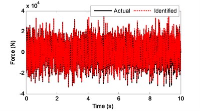
Fig. 2Zoom-in view of a segment (2-2.4 s) of Fig. 1

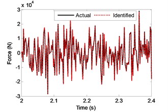
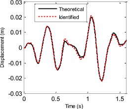
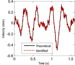
Fig. 3a) The theoretical and identified displacement at the 2nd floor, b) the theoretical and identified velocity at the 2nd floor

a)

b)

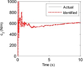
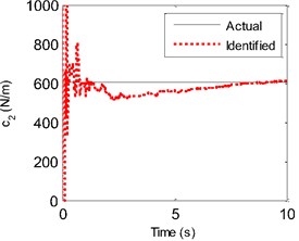
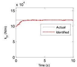
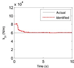
Fig. 4a) The actual and identified parameter value of c2, b) the actual and identified parameter value of c3, c) the actual and identified parameter value of k21, d) The actual and identified parameter value of k31

a)

b)

c)

d)

And to make a clearer comparison, the segment history of the actual and identified excitations from 2 s-2.4 s is also shown in Fig. 2. Then, the identified displacement and velocity responses at the 2nd floor are compared with their corresponding theoretical values as shown in Fig. 3. From Fig. 1 to Fig. 3, one can know that the identified force and structural state are both accurate. Also, the four identified parameters are plotted in Fig. 4. At the beginning of the identified procedure, the identified parameter values have the strong oscillatory, and then are quickly convergent to the neighborhoods of their corresponding actual values. From the above comparisons, it is clear that the proposed EGDF algorithm has the ability for simultaneous excitation and parameter identification for the non-linear Duffing-type system.

4.2. Example 2: 4-DOF hysteretic structure with time-varying parameters

The other numerical example is to identify the hysteretic parameters of a four-story hysteretic shear-beam building subject to unmeasured excitation on the top floor of the building, as shown by Fig. 5.

Fig. 5A hysteric shear-frame building under unknown excitation

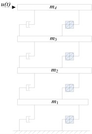
The equations of motion are given as:

where $\mathbf{r}\left(t\right)$ is the vector of hysteretic force with $r_i\left(t\right)$($i=$ 1, 2,…, 4) being the $i$th floor hysteretic restoring force and is herein modeled by the Bouc-Wen non-linear differential equation, which can be written as:

where ${\theta }_i$, ${\beta }_i$, ${\gamma }_i$ and ${\alpha }_i$ are the Bouc-Wen hysteretic parameters. The hysteretic force is hereditary, depending on the past history of deformation, and its description is very complicated. Thus, the structure is non-linear. Structural hysteretic performance can be used as the indicator of the development of structural damage under dynamic excitation. Therefore, structure damage can be detected based on the identification of hysteretic parameters.

The following parameters are used in the example: mass of each of each floor $m_1=m_2=m_3=m_4=\text{500}$ kg; each story stiffness $k_1=k_2=k_3=k_4=\text{24}$ kN/m; each story damping coefficients $c_1=c_2=c_3=c_4=$ 0.1 kNs/m; hysteretic parameters are time-varying, and have the relations as ${\theta }_1={\theta }_2={\theta }_3={\theta }_4\text{,}$${\beta }_1={\beta }_2={\beta }_3={\beta }_4\text{,}$${\gamma }_1={\gamma }_2={\gamma }_3={\gamma }_4\text{,}$${\alpha }_1={\alpha }_2={\alpha }_3={\alpha }_4$. The external excitation on the 4th floor is assumed to be a white noise force. The response time histories of the non-linear structure are calculated by the Runge-Kutta method. Three acceleration responses at the 1st, 3rd and 4th floors are assumed to be measured. The influence of measurement noise on identification is considered by superimposition of noise process with the computed response quantities. In this example, 3 % RMS noise are adopted. The external excitation applied on the 4th floor is assumed to be unknown for identification.

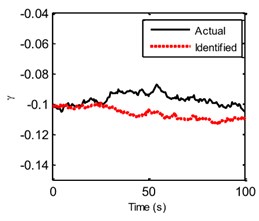
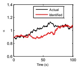
In the EGDF algorithm, the unknown quantities to be identified are the augmented state vector $\mathbf{z}=\{\mathbf{p},\dot{\mathbf{p}},\mathbf{r},\theta ,\beta ,\gamma ,\alpha \}$ and the unmeasured external excitation $u\left(t\right)$. The sampling time interval is 0.5 s. Based on the algorithm, the unmeasured excitation, displacement, velocity, hysteretic forces and hysteretic parameters can be identified. Fig. 6 shows the curves of the actual and identified excitations, and Fig. 7 is the segment view of Fig. 6 from 0 s to 40 s, which is to make a clearer comparison. The identified structural state of the 2nd floor is plotted in Fig. 8 compared with the responding theoretical value. The identified velocity response is very accurate, and the identified displacement response is also accurate with a minor error. The identified hysteretic force between 3rd and 4th floor is plotted in Fig. 9. The identified error occurs mainly due to the error of the identified displacement. The identified time-varying non-linear parameters are shown in Fig. 10. The dashed lines marked in red represent the up and bottom boundaries of the identified parameters. From all the above figures, it demonstrates that the proposed EGDF approach is capable of simultaneous excitation and parameter identification for non-linear Bouc-Wen hysteretic systems.

Fig. 6The actual and identified results of random force ut

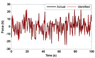
Fig. 7Zoom-in view of a segment (0-40 s) of Fig. 6

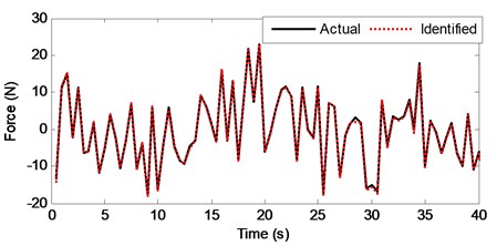
Fig. 8a) The theoretical and identified displacement of the vertical direction at the 2nd floor, b) the theoretical and identified velocity of the vertical direction at the 2nd floor

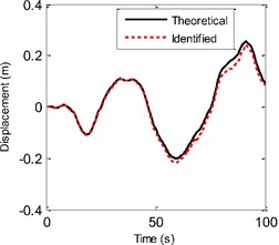
a)

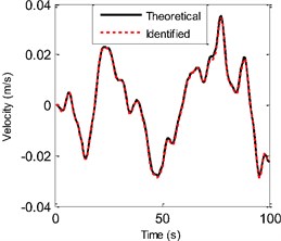
b)

Fig. 9The theoretical and identified hysteretic force between the 3rd and 4th floors

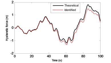
Fig. 10The actual and identified hysteretic parameters

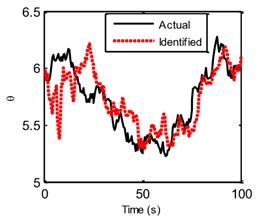
a)

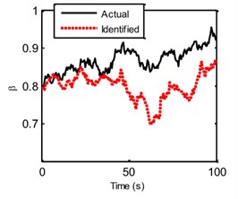
b)

c)

d)