Extension of piecewise exact solution method for two- and three-dimensional fluid flows

Kim, Hyoseob; Ahn, Jongsup; Jang, Changhwan; Jin, Jaeyoull; Jung, Byungsoon

Journal of Vibroengineering

Browse Journal

Submit article

Published: 30 September 2013

Check for updates

Extension of piecewise exact solution method for two- and three-dimensional fluid flows

Hyoseob Kim¹

Jongsup Ahn²

Changhwan Jang³

Jaeyoull Jin⁴

Byungsoon Jung⁵

^{1, 2}Kookmin University, Seoul, Korea

³Korean Intellectual Property Office, Daejeon, Korea

⁴Korea Institute of Ocean Science & Technology (KIOST), Ansan, Korea

⁵Sea & River Consultant Inc., Seoul, Korea

Corresponding Author:

Changhwan Jang

Cite the article Download PDF

Downloads 1211

Abstract

Extended forms of a pseudo-numerical scheme for advection terms in fluid momentum equations are proposed here. The fact that analytic solution exists for the Burgers equation, if velocity distribution in space is straight for one-dimensional flow, was shown by Jang et al. Analytic solution also exists for two- or three-dimensional fluid flows, if the velocity components in two- or three-direction are linearly distributed in space, and the existing piecewise exact solution method is extended for two- and three-dimensions here. The analytic solution is adopted for computation of the advecting property of fluid momentum in two- or three-dimensional directions. This method produces zero numerical error during one time increment so that it is distinguished from any other numerical scheme which produces small or large numerical error within one time increment. The behavior of the new scheme is demonstrated for two- and three-dimensional examples. The nonlinear modifications of velocity profiles towards singularity with time progress are well simulated for three test cases. The computed maximum relative errors for a given condition for one-, two-, and three-dimensions become larger as the number of dimension increases. The scheme is believed to work well for two- and three-dimensional flows.

1. Introduction

Fluid motion is governed by conservation equations including momentum conservation equation. Not only the advection equation but also the advection-diffusion equation has been intensively used to describe the flow of fluids or other material in engineering problems [1, 2, 3].

Fundamentally, the one-dimensional advection-diffusion equation has a form:

1

\frac{\partial u}{\partial t} + a \frac{\partial u}{\partial t} = v \frac{\partial^{2} u}{\partial x^{2}},

which is reduced to the advection-only equation:

2

\frac{\partial u}{\partial t} + a \frac{\partial u}{\partial x} = 0,

where $a$ is the transporting celerity, and $u$ is a physical property. The inviscid Burgers equation is a specific form of the above advection equation, when $a = u$ :

3

\frac{\partial u}{\partial t} + u \frac{\partial u}{\partial x} = 0 .

From mathematical point of view the momentum equations in three dimensions are composed of several terms, i.e, advection terms, diffusion terms, and the others. Fractional step method [4, 5] or operator splitting method [6] is often adopted in numerical solution procedure due to its convenience and simplicty. The one-dimensional invisicid Burgers equation can be written in conservative form as:

4

\frac{\partial u}{\partial t} + \frac{\partial F (u)}{\partial x} = 0,

5

F (u) = \frac{u^{2}}{2},

where $x$ is the spatial axis, $t$ is the time, and $u$ is the velocity in the $x$ axis. The velocity field $u (x, t)$ at the initial time $(t = 0)$ is $u (x, 0)$ and is called $f (x_{0})$ . The analytic solution of Eq. (4) for the given initial condition is:

6

u_{L} (x_{0}, t) = u (x_{0}, 0) = f (x_{0}),

where $u_{L}$ is the velocity for Langrangean position. The Eulerian description of the velocity becomes:

7

x = x_{0} + u_{L} \cdot t = x_{0} + f (x_{0}) \cdot t,

8

u (x, t) = u (x_{0} + f (x_{0}) \cdot t, t) = u_{L} (x_{0}, t) = u_{L} (x_{0}, 0) = f (x_{0}) .

The above advection equation is called the inviscid Burgers equation [7, 8]. The two- or three-dimensional Burgers equation in a Lagrangean form is:

9

D V / D t = 0,

where $V$ is the velocity vector of fluid flow, $V = (u, v, w)$ , $(u, v)$ , or $(u)$ for three-dimensional, two-dimensional, or one-dimensional flow, respectively, where $u$ , $v$ and $w$ are the velocity components in the $x$ , $y$ and $z$ directions, respectively. Eulerian forms of the Burgers equations are then:

10

\frac{\partial u}{\partial t} + u \frac{\partial u}{\partial x} + v \frac{\partial u}{\partial y} + w \frac{\partial u}{\partial z} = 0,

\frac{\partial v}{\partial t} + u \frac{\partial v}{\partial x} + v \frac{\partial v}{\partial y} + w \frac{\partial v}{\partial z} = 0,

\frac{\partial w}{\partial t} + u \frac{\partial w}{\partial x} + v \frac{\partial w}{\partial y} + w \frac{\partial w}{\partial z} = 0 .

The problem is that it is not always possible to get the solution in an explict form for an arbitrary initial function $f$ . We need adquate nemerical methods which are good for fixed grid system [9, 10]. One of frequently used numerical schemes to solve the advection equation is the upwind scheme [9]:

11

\frac{u_{i}^{n + 1} + u_{i}^{n}}{Δ t} = - \frac{{\bar{u}}_{i}^{n}}{Δ x} (u_{i + 1}^{n} - u_{i}^{n} or u_{i}^{n} - u_{i - 1}^{n}),

where superscript $n$ or $n + 1$ means the time step $n$ or $n + 1$ , subscript $i$ means the spatial grid number $i$ , ${\bar{u}}_{i}^{n}$ is a representative velocity at the index number $i$ at time step $n$ , which could either be $u_{i}^{n}$ , $u_{i + 1}^{n}$ , $u_{i - 1}^{n}$ , $(u_{i}^{n} + u_{i + 1}^{n}) / 2$ or $(u_{i - 1}^{n} + u_{i}^{n}) / 2$ . If we use the difference equation for the Burgers equation in the conservative form, the difference equation becomes:

12

\frac{u_{i}^{n}}{Δ t} = - \frac{1}{2 Δ x} \{{(u_{i + 1}^{n})}^{2} - {(u_{i}^{n})}^{2} or {(u_{i}^{n})}^{2} - {(u_{i - 1}^{n})}^{2}\} .

This virtually takes a representative velocity as $(u_{i}^{n} + u_{i + 1}^{n}) / 2$ or $(u_{i - 1}^{n} + u_{i}^{n}) / 2$ depending on the flow direction. Jang et al. [12] proposed a useful piecewise exact solution method (PESM) to solve the one-dimensional advection equation, Eq. (3). If the velocity is linearly distributed in space as:

13

u = \frac{x + c}{t} .

Then the above equation itself satisfies the advection equation, Eq. (3), if conditions are well-posed. Eq. (13) may have a singular solution, if the velocity gradient becomes infinity as time goes by. This corresponds to shock wave in physical domain [11]. The solution at a fixed point of index $i$ becomes:

14

u_{i}^{n + 1} = \frac{Δ x}{(u_{i}^{n} - u_{i - 1}^{n}) Δ t + Δ x} u_{i}^{n} .

However, if the governing momentum equation is to be solved with the splitting method, the analytical solution for some long period may not be very useful, because not only invisid Burgers equation but also the diffusion equation or other equation with other terms should be alternately solved every time step. Therefore the analytical solution for the invisid Burgers equation may be useful for each time increment only.

Interesting feature of this solution is that the orgin of $t$ , $t_{0}$ is not a priori, but should be found, and the solution is not temporarilly linear from the Eulerion point of view. If a fixed grid is used, and two velocities, at two points $x_{i}$ and $x_{i - 1}$ at time $t_{0}$ are:

15

u_{i}^{n} = \frac{x_{i} + c}{t_{0}}, u_{i - 1}^{n} = \frac{x_{i} - Δ x + c}{t_{0}} .

We can remove $c$ from Eq. (15), and get $u_{i}^{n + 1}$ as:

16

u_{i}^{n + 1} = \frac{x_{i} + c}{t_{0} + Δ t} = \frac{Δ x u_{i}^{n}}{(u_{i}^{n} - u_{i - 1}^{n}) Δ t + Δ x} .

If the velocity at $x_{i}$ is negative, the velocity at $x_{i}$ at new time step is:

17

u_{i}^{n + 1} = \frac{Δ x u_{i}^{n}}{(u_{i + 1}^{n} - u_{i}^{n}) Δ t + Δ x} .

The above PESM for one-dimensional advection equation was compared with Godunov's method [11], and demonstrated higher accuracy relative to Godunov's method. Since the above solution is the analytic solution, it does not produce any numerical error during a time increment, but errors develop during the spatial interpolation. The PESM was compared with a few existing numerical schemes, and showed unconditional stability for CFL number larger than 1.0 by using the following extended solution:

18

\begin{matrix} u_{i}^{n + 1} = \frac{Δ x {(m + 1) u_{i - m}^{n} - m u_{i - m - 1}^{n}}}{(u_{i - m}^{n} - u_{i - m - 1}^{n}) Δ t + Δ x}, u_{i}^{n} \geq 0 a n d u_{i - m}^{n} Δ t \geq m Δ x, \\ u_{i}^{n + 1} = \frac{Δ x {(m + 1) u_{i - m}^{n} - m u_{i - m + 1}^{n}}}{(u_{i - m + 1}^{n} - u_{i - m}^{n}) Δ t + Δ x}, u_{i}^{n} < 0 a n d u_{i - m}^{n} Δ t < m Δ x, \end{matrix}

where $m$ is an integer. Jang et al. suggested the above solutions could be used for the first-order portion of any other existing higher order schemes, e.g. Fromm's or Lax-Wenddroff scheme. However, Jang et al.’s method has been confined to one-dimensional form.

2. Extension of PESM for two- and three-dimensional cases

We are extending Jang et al.’s PESM for higher dimension here, i.e. for two-dimensional and three-dimensional advection equations [12]. Starting from one-dimensional problem, we adopt coefficients for spacial distribution of velocity, not involving $t_{0}$ :

19

u_{i}^{n} = a x_{i} + b,

u_{i - 1}^{n} = a (x_{i} - Δ x) + b,

where $b$ implicity include the time effect. We can also use the invariant Lagrangean advection property of the velocity component. Furthermore we also know that the solution must be spatially linear:

20

u_{i}^{n + 1} = d x_{i} + e .

We have two boundary values at two points at the advanced time:

21

u_{i^{*}}^{n + 1} = u_{i}^{n} at x_{i^{*}} = x_{i} + u_{i}^{n} Δ t,

u_{{(i - 1)}^{*}}^{n + 1} = u_{i - 1}^{n} at x_{{(i - 1)}^{*}} = x_{i - 0} - Δ x + u_{i - 1}^{n} Δ t,

where superscript ^* means the new position of the particle which was at grid point $i$ at the previous time. Inserting Eq. (21) into Eq. (19), we obtain the solution for $u_{i}^{n + 1}$ which is identical to Eq. (16). Now we expand this approach to the two-dimensional advection equations:

22

\frac{\partial u}{\partial t} = u \frac{\partial u}{\partial x} + v \frac{\partial u}{\partial y},

\frac{\partial v}{\partial t} = u \frac{\partial v}{\partial x} + v \frac{\partial v}{\partial y} .

A rectangular grid is considered at this stage. Planar distribution of the two velocity components at an instance are assumed as:

23

u = \frac{a_{1} x + a_{2} y + a_{3}}{t}, v = \frac{b_{1} x + b_{2} y + b_{3}}{t},

24

u (x, y, t_{0}) = \frac{a_{1} x + a_{2} y + a_{3}}{t_{0}} = c_{1} x + c_{2} y + c_{3}, v (x, y, t_{0}) = d_{1} x + d_{2} y + d_{3} .

The coefficients $a_{1}$ , $a_{2}$ , $a_{3}$ , $b_{1}$ , $b_{2}$ , $b_{3}$ are assumed to satisfy Eq. (22). We have six boundary values at three triangle corner points $A$ , $B$ and $C$ of a triangle at time $t_{0}$ . For example, if $u_{i, j}^{n} \geq 0$ and $v_{i, j}^{n} \geq 0$ , then the three corner points will move to other positions ${(i, j)}^{*}$ , ${(i - 1, j)}^{*}$ and ${(i, j - 1)}^{*}$ at $t_{0} + Δ t$ :

25

u_{{(i, j)}^{*}}^{n + 1} = c_{1} x_{{(i, j)}^{*}} + c_{2} y_{{(i, j)}^{*}} + c_{3},

u_{{(i - 1, j)}^{*}}^{n + 1} = c_{1} x_{{(i - 1, j)}^{*}} + c_{2} y_{{(i - 1, j)}^{*}} + c_{3},

u_{{(i, j - 1)}^{*}}^{n + 1} = c_{1} x_{{(i, j - 1)}^{*}} + c_{2} y_{{(i, j - 1)}^{*}} + c_{3},

26

v_{{(i, j)}^{*}}^{n + 1} = d_{1} x_{{(i, j)}^{*}} + d_{2} y_{{(i, j)}^{*}} + d_{3},

v_{{(i - 1, j)}^{*}}^{n + 1} = d_{1} x_{{(i - 1, j)}^{*}} + d_{2} y_{{(i - 1, j)}^{*}} + d_{3},

v_{{(i, j - 1)}^{*}}^{n + 1} = d_{1} x_{{(i, j - 1)}^{*}} + d_{2} y_{{(i, j - 1)}^{*}} + d_{3},

where:

27

x_{{(i, j)}^{*}}^{n + 1} = u_{(i, j)}^{n} Δ t,

y_{{(i, j)}^{*}}^{n + 1} = v_{(i, j)}^{n} Δ t,

28

x_{{(i - 1, j)}^{*}}^{n + 1} = - Δ x + u_{(i - 1, j)}^{n} Δ t,

y_{{(i - 1, j)}^{*}}^{n + 1} = v_{(i - 1, j)}^{n} Δ t,

29

x_{{(i, j - 1)}^{*}}^{n + 1} = u_{(i, j - 1)}^{n} Δ t,

y_{{(i, j - 1)}^{*}}^{n + 1} = - Δ y + v_{(i, j - 1)}^{n} Δ t .

Fig. 1Position movement of three corner points of triangle for 2-dimensional case

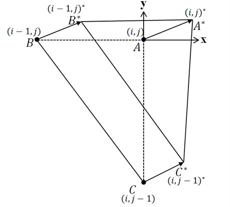
Then, at time $t_{0} + Δ t$ the six unknowns $c_{1}$ , $c_{2}$ , $c_{3}$ , $d_{1}$ , $d_{2}$ , $d_{3}$ are obtained from the above six equations. For different flow directions other three corner points are chosen, i.e. $(i, j)$ , $(i - 1, j)$ , $(i, j + 1)$ for negative $u_{i, j}$ and positive $v_{i, j}$ , and $(i, j)$ , $(i + 1, j)$ , $(i, j + 1)$ for positive $u_{i, j}$ and negative $v_{i, j}$ . Eqs. (27) to (29) can be expressed as:

30

M_{1} c = u,

M_{2} d = v,

where $M_{1}$ , $M_{2}$ are the coefficient matrices, $c$ and $d$ are the unknown vectors $(c_{1}, c_{2}, c_{3})$ and $(d_{1}, d_{2}, d_{3})$ , respectively; $u$ and $v$ are known boundary value vector $(u_{{(i, j)}^{*}}^{n + 1}, u_{{(i - 1, j)}^{*}}^{n + 1}, u_{{(i, j - 1)}^{*}}^{n + 1})$ and $(v_{{(i, j)}^{*}}^{n + 1}, v_{{(i - 1, j)}^{*}}^{n + 1}, v_{{(i, j - 1)}^{*}}^{n + 1})$ , respectively. Then:

31

c = {M_{1}}^{- 1} u

d = {M_{2}}^{- 1} v .

Thus $u_{i, j}^{n + 1} = c_{3}$ and $v_{i, j}^{n + 1} = d_{3}$ are new velocity components at $(i, j)$ , i.e. $x = y = 0$ . Next we expand this approach to the three-dimensional advection equations:

32

\frac{\partial u}{\partial t} = u \frac{\partial u}{\partial x} + u \frac{\partial u}{\partial y} + u \frac{\partial u}{\partial z},

\frac{\partial v}{\partial t} = v \frac{\partial v}{\partial x} + v \frac{\partial v}{\partial y} + v \frac{\partial v}{\partial z},

\frac{\partial w}{\partial t} = w \frac{\partial w}{\partial x} + w \frac{\partial w}{\partial y} + w \frac{\partial w}{\partial z} .

A rectangular parallelepiped grid is considered at this stage. Planar distribution of the three velocity components at an instance are assumed as:

33

u = \frac{a_{1} x + a_{2} y + a_{3} z + a_{4}}{t}, v = \frac{b_{1} x + b_{2} y + b_{3} z + b_{4}}{t}, w = \frac{c_{1} x + c_{2} y + c_{3} z + c_{4}}{t},

34

u (x, y, z, t_{0}) = d_{1} x + d_{2} y + d_{3} z + d_{4},

v (x, y, z, t_{0}) = e_{1} x + e_{2} y + e_{3} z + e_{4},

w (x, y, z, t_{0}) = f_{1} x + f_{2} y + f_{3} z + f_{4} .

The coefficients $a_{1}$ , $a_{2}$ , $a_{3}$ , $a_{4}$ , $b_{1}$ , $b_{2}$ , $b_{3}$ , $b_{4}$ , $c_{1}$ , $c_{2}$ , $c_{3}$ , $c_{4}$ are assumed to satisfy Eq. (32). We have twelve boundary values at four corner points $A$ , $B$ , $C$ and $D$ of the quadrangular pyramid at time $t_{0}$ . For example, if $u_{i, j}^{n} \geq 0$ , $v_{i, j}^{n} \geq 0$ and $w_{i, j}^{n} \geq 0$ then the four corner points will take other positions at $t_{0} + Δ t$ :

35

u_{{(i, j, k)}^{*}}^{n + 1} = c_{1} x_{{(i, j, k)}^{*}} + c_{2} y_{{(i, j, k)}^{*}} + c_{3} z_{{(i, j, k)}^{*}} + c_{4},

u_{{(i - 1, j, k)}^{*}}^{n + 1} = c_{1} x_{{(i - 1, j, k)}^{*}} + c_{2} y_{{(i - 1, j, k)}^{*}} + c_{3} z_{{(i - 1, j, k)}^{*}} + c_{4},

u_{{(i, j - 1, k)}^{*}}^{n + 1} = c_{1} x_{{(i, j - 1, k)}^{*}} + c_{2} y_{{(i, j - 1, k)}^{*}} + c_{3} z_{{(i, j - 1, k)}^{*}} + c_{4},

u_{{(i, j, k - 1)}^{*}}^{n + 1} = c_{1} x_{{(i, j, k - 1)}^{*}} + c_{2} y_{{(i, j, k - 1)}^{*}} + c_{3} z_{{(i, j, k - 1)}^{*}} + c_{4},

36

v_{{(i, j, k)}^{*}}^{n + 1} = d_{1} x_{{(i, j, k)}^{*}} + d_{2} y_{{(i, j, k)}^{*}} + d_{3} z_{{(i, j, k)}^{*}} + d_{4},

v_{{(i - 1, j, k)}^{*}}^{n + 1} = d_{1} x_{{(i - 1, j, k)}^{*}} + d_{2} y_{{(i - 1, j, k)}^{*}} + d_{3} z_{{(i - 1, j, k)}^{*}} + d_{4},

v_{{(i, j - 1, k)}^{*}}^{n + 1} = d_{1} x_{{(i, j - 1, k)}^{*}} + d_{2} y_{{(i, j - 1, k)}^{*}} + d_{3} z_{{(i, j - 1, k)}^{*}} + d_{4},

v_{{(i, j, k - 1)}^{*}}^{n + 1} = d_{1} x_{{(i, j, k - 1)}^{*}} + d_{2} y_{{(i, j, k - 1)}^{*}} + d_{3} z_{{(i, j, k - 1)}^{*}} + d_{4},

37

w_{{(i, j, k)}^{*}}^{n + 1} = a_{1} x_{{(i, j, k)}^{*}} + a_{2} y_{{(i, j, k)}^{*}} + a_{3} z_{{(i, j, k)}^{*}} + a_{4},

w_{{(i - 1, j, k)}^{*}}^{n + 1} = a_{1} x_{{(i - 1, j, k)}^{*}} + a_{2} y_{{(i - 1, j, k)}^{*}} + a_{3} z_{{(i - 1, j, k)}^{*}} + a_{4},

w_{{(i, j - 1, k)}^{*}}^{n + 1} = a_{1} x_{{(i, j - 1, k)}^{*}} + a_{2} y_{{(i, j - 1, k)}^{*}} + a_{3} z_{{(i, j - 1, k)}^{*}} + a_{4},

w_{{(i, j, k - 1)}^{*}}^{n + 1} = a_{1} x_{{(i, j, k - 1)}^{*}} + a_{2} y_{{(i, j, k - 1)}^{*}} + a_{3} z_{{(i, j, k - 1)}^{*}} + a_{4},

where:

38

x_{{(i, j, k)}^{*}}^{n + 1} = u_{(i, j, k)}^{n} Δ t,

y_{{(i, j, k)}^{*}}^{n + 1} = v_{(i, j, k)}^{n} Δ t,

z_{{(i, j, k)}^{*}}^{n + 1} = w_{(i, j, k)}^{n} Δ t,

39

x_{{(i - 1, j, k)}^{*}}^{n + 1} = - Δ x + u_{(i - 1, j, k)}^{n} Δ t,

y_{{(i - 1, j, k)}^{*}}^{n + 1} = v_{(i - 1, j, k)}^{n} Δ t,

z_{{(i - 1, j, k)}^{*}}^{n + 1} = w_{(i - 1, j, k)}^{n} Δ t,

40

x_{{(i, j - 1, k)}^{*}}^{n + 1} = u_{(i, j - 1, k)}^{n} Δ t,

y_{{(i, j - 1, k)}^{*}}^{n + 1} = - Δ y + v_{(i, j - 1, k)}^{n} Δ t,

z_{{(i, j - 1, k)}^{*}}^{n + 1} = w_{(i, j - 1, k)}^{n} Δ t,

41

x_{{(i, j, k - 1)}^{*}}^{n + 1} = u_{(i, j, k - 1)}^{n} Δ t,

y_{{(i, j, k - 1)}^{*}}^{n + 1} = v_{(i, j, k - 1)}^{n} Δ t,

z_{{(i, j, k - 1)}^{*}}^{n + 1} = - Δ z + w_{(i, j, k - 1)}^{n} Δ t .

Fig. 2Position movement of four corner points of quadangular pyramid for 3-dimensional case

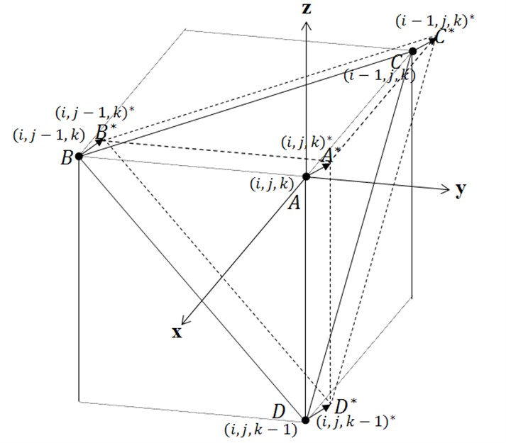
Then, at time $t_{0} + Δ t$ the twelve unknown coefficients $d_{1}$ , $d_{2}$ , $d_{3}$ , $d_{4}$ , $e_{1}$ , $e_{2}$ , $e_{3}$ , $e_{4}$ , $f_{1}$ , $f_{2}$ , $f_{3}$ , $f_{4}$ are obtained from the above twelve equations. For different flow directions from the above case, other four corner points are chosen, see Table 1. Eqs. (35) to (37) can be expressed as:

42

M_{1} d = u,

M_{2} e = v,

M_{3} f = w,

where $M_{1},$ $M_{2},$ $M_{3}$ are the coefficient matrices, $d,$ $e$ and $f$ are the unknown vectors $(d_{1}, d_{2}, d_{3}, d_{4})$ , $(e_{1}, e_{2}, e_{3}, e_{4})$ , $(f_{1}, f_{2}, f_{3}, f_{4})$ respectively, and $u$ , $v$ and $w$ are known boundary value vectors $(u_{{(i, j, k)}^{*}}^{n + 1}, u_{{(i - 1, j, k)}^{*}}^{n + 1}, u_{{(i, j - 1, k)}^{*}}^{n + 1}, u_{{(i, j, k - 1)}^{*}}^{n + 1})$ , $(v_{{(i, j, k)}^{*}}^{n + 1}, v_{{(i - 1, j, k)}^{*}}^{n + 1}, v_{{(i, j - 1, k)}^{*}}^{n + 1}, v_{{(i, j, k - 1)}^{*}}^{n + 1})$ and $(w_{{(i, j, k)}^{*}}^{n + 1}, w_{{(i - 1, j, k)}^{*}}^{n + 1}, w_{{(i, j - 1, k)}^{*}}^{n + 1}, w_{{(i, j, k - 1)}^{*}}^{n + 1})$ respectively. Then:

43

d = {M_{1}}^{- 1} u

e = {M_{2}}^{- 1} v,

f = {M_{3}}^{- 1} w

Thus, $u_{i, j, k}^{n + 1} = d_{3},$ $v_{i, j, k}^{n + 1} = e_{3}$ and $w_{i, j, k}^{n + 1} = f_{3}$ are new velocity components at $(i, j, k),$ i.e. $x = y = z = 0$ .

Table 1Selection of four corner points for different signs of u, v and w

$u_{i, j, k}$	$v_{i, j, k}$	$w_{i, j, k}$	Four points
+	+	-	$(i, j, k), (i - 1, j, k), (i, j - 1, k), (i, j, k + 1)$
+	-	+	$(i, j, k), (i - 1, j, k), (i, j + 1, k), (i, j, k - 1)$
+	-	-	$(i, j, k), (i - 1, j, k), (i, j + 1, k), (i, j, k + 1)$
-	+	+	$(i, j, k), (i + 1, j, k), (i, j - 1, k), (i, j, k - 1)$
-	+	-	$(i, j, k), (i + 1, j, k), (i, j - 1, k), (i, j, k + 1)$
-	-	+	$(i, j, k), (i + 1, j, k), (i, j + 1, k), (i, j, k - 1)$
-	-	-	$(i, j, k), (i + 1, j, k), (i, j + 1, k), (i, j, k + 1)$

3. Examinations of present extention

Now we apply the present PESM extended for two- and three-dimensional fluid flow to two simple two- and three-dimensional situations. The initial distribution of the velocity field of the the two- dimensional flow is given as:

44

u = \frac{\sqrt{2}}{2} \{1 + e x p (\frac{- {(x - 50)}^{2} - {(y - 50)}^{2}}{500})\},

v = \frac{\sqrt{2}}{2} \{1 + e x p (\frac{- {(x - 50)}^{2} - {(y - 50)}^{2}}{500})\} .

And the initial velocity field for a simple three-dimensional situation is:

45

u = \frac{\sqrt{3}}{3} \{1 + e x p (\frac{- {(x - 50)}^{2} - {(y - 50)}^{2} - {(z - 50)}^{2}}{500})\},

v = \frac{\sqrt{3}}{3} \{1 + e x p (\frac{- {(x - 50)}^{2} - {(y - 50)}^{2} - {(z - 50)}^{2}}{500})\},

w = \frac{\sqrt{3}}{3} \{1 + e x p (\frac{- {(x - 50)}^{2} - {(y - 50)}^{2} - {(z - 50)}^{2}}{500})\} .

Fig. 3Speed contour at two instants for two dimensional test flow: t=0

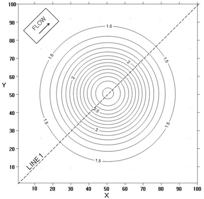
Fig. 4Speed contour at two instants for two dimensional test flow: t=15

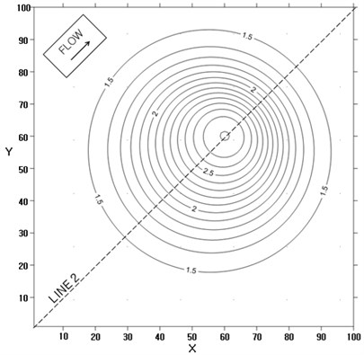
Fig. 5Speed contour at two instants for three dimensional test flow: t= 0

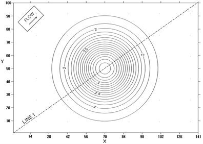
Fig. 6Speed contour at two instants for three dimensional test flow: t= 15

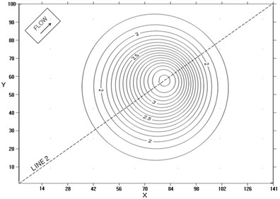
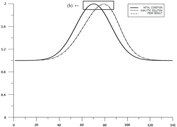
Fig. 7Velocity profiles along x axis for one-dimensional flow

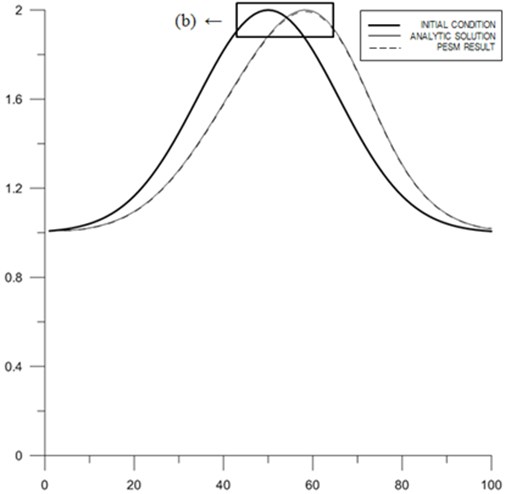
a) Profile

b) Zoomed view

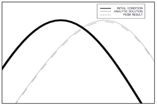
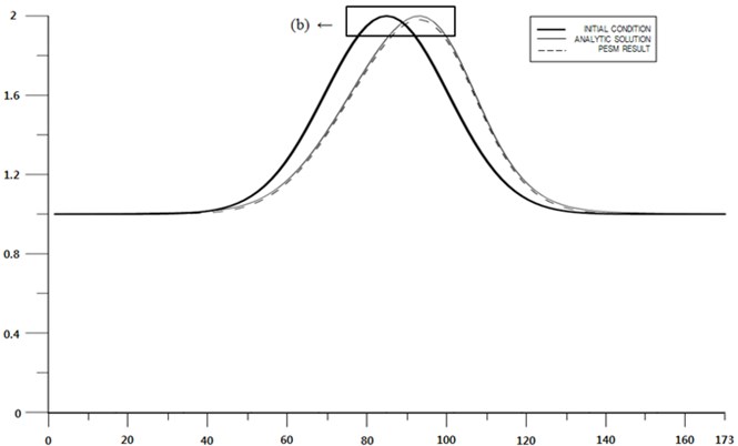
Fig. 8Velocity profiles along x axis for two-dimensional flow

a) Profile

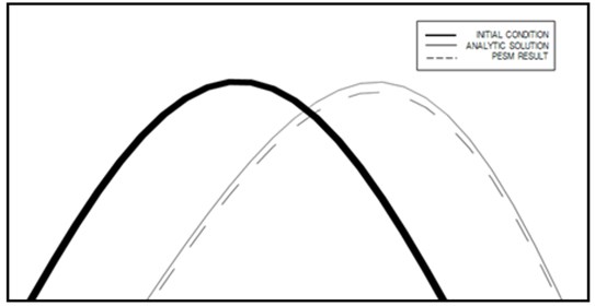
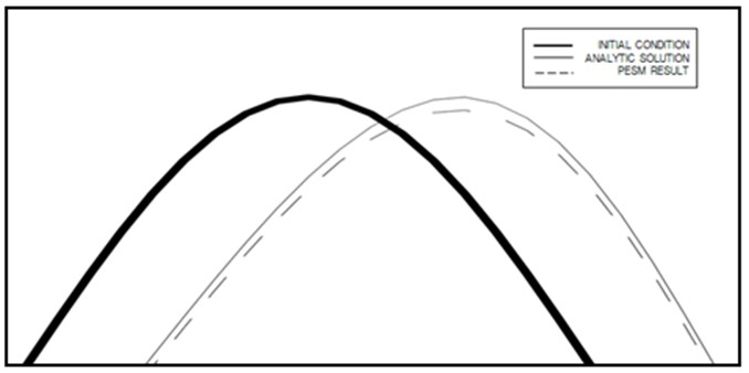
b) Zoomed view

One-dimensional case is also used for comparision with the two- and three-dimensional cases. The initial velocity distribution of the one-dimensional case is:

46

u = 1 + e x p (\frac{- {(x - 50)}^{2}}{500}) .

The application results of this method to the two-dimensional and three-dimensional progressive flood cases are shown in Figs. 3, 4, 5 and 6, respectively.

Computed profiles of the speed along central lines at two instants for one-, two-, and three-dimensional cases are shown in Figs. 7 to 9. Figs. 7 to 9 show that even though the PESM is the exact solution for each $Δ t$ , the method still produces numerical diffusion due to the process of spacial interpolation every time step, see Jang et al. [12]. The computed distributions of speed along central lines are close to analytical solution for one-, two-, and three-dimensional cases, respectively. The maximum relative errors of the computed speed for one-, two-, and three-dimensional cases are shown in Table 2. The relative error becomes larger as the number of dimensions increases, which means the spacial interpolation produces high diffusion. Nontheless the expanded PESM works well for two-and three-dimensional problems according to the present examinations.

Fig. 9Velocity profiles along x axis for three-dimensional flow

a) Profile

b) Zoomed view

Table 2Comparison of relative errors for different dimensions

Dimension	Analytic solution	PESM result	Relative error (%)
One	2.0000	1.9931	0.3457
Two	2.0000	1.9844	0.7799
Three	2.0000	1.9812	0.9408

4. Conclusions

Previous PESM for one-dimensional flow was expanded here for two-, and three-dimensional fluid flows. The PESM takes exact solution within one time step and therefore it is irrelevant to any numerical error, although it is not free from interpolation error due to the non-moving property of grid computational. The PESM secures unconditional stability, which is important for practical use in numerical modeling workes. Algorithms for two- or three-dimensional advection equations are extensions of that for one-dimensional advection equation. The boundery values at corners of a triangle or a quadrangular pyramid at time $t_{0}$ preserved at time $t_{0} + Δ t$ according to the characteristics of the Lagrangean advection equation. The method was applied to simple situations, and the results are satisfactory. The diffusion due to spacial interpolation become larger as the dimension becomes larger. The PESM is believed to work well for arbitrary number of dimensions.

References

Morton K. W., Mayers D. F. Numerical Solution of Partial Differential Equations. Cambridge University Press, Cambridge, UK, 2005, p. 86-150.

Search CrossRef
Ibragimov N. H. Handbook of Lie Groups to Analysis of Differential Equations. Vol. 1, CRC Press, Boca Raton, USA, 1994.

Search CrossRef
Polyanin A. D., Zaitsev V. F. Handbook of Nonlinear Partial Differential Equations. Chapman and Hall / CRC, Boca Raton, USA, 2004.

Search CrossRef
Perot J. B. An analysis of the fractional step method. J. of Comput. Phys., Vol. 108, 1993, p. 51-58.

Search CrossRef
Armfiled S., Street R. Modified fractional-step methods for the Navier-Stokes equations. ANZIAM J., Vol. 45, 2004, p. 364-377.

Search CrossRef
Karlsen K. H., Risebro N. H. An operator splitting method for nonlinear convection-diffusion equation. Number. Math., Vol. 77, No. 3, 1994, p. 365-382.

Search CrossRef
Burgers J. M. The Nonlinear Diffusion Equation. Reidel, Dordreht, Netherlands, 1974.

Search CrossRef
Burgers J. M. A mathematical model illustrating the theory of turbulence. Adv. Appl. Meth., Vol. 1, 1948, p. 171-199.

Search CrossRef
Welch J. E., Harlow F. H., Shannon J. P., Daly B. J. The MAC Method. Los Alamos Scientific Lab. Rept. LA-3425, Los Alamos, New Mexico, USA, 1966.

Search CrossRef
Fromm J. E. A method for reducing dispersion in convective difference schemes. J. Comput. Phys., Vol. 3, 1968, p. 176-189.

Search CrossRef
Godunov S. K. A difference scheme for numerical solution of discontinuous solution of hydrodynamic equations. Math. Sbornik, Vol. 47, 1989, p. 271-306.

Search CrossRef
Jang C., Kim H., Choi C., Kim J. Piecewise exact solution of nonlinear momentum conservation equation with unconditional stability for time increment. Journal of Vibroengineering, Vol. 14, 2012, p. 1041-1051.

Search CrossRef
Lax P. D., Wendroff B. Systems of conservation laws. Comm. Pure Appl. Math., Vol. 13, No. 2, 1960, p. 217-237.

Search CrossRef
Sarra S. A. The method of characteristics with application to conservation laws. J. of Online Math. and Its Appl., Vol. 3, 2003.

Search CrossRef
Roe P. L. Approximate Riemann solvers, parameter vectors, and difference schemes. J. of Comput. Phys., Vol. 43, 1981, p. 357-372.

Search CrossRef
Harten A. One class of high resolution total-variation-stable finite difference schemes. SIAM J. Numer. Anal., Vol. 21, 1984, p. 1-23.

Search CrossRef
Thomee V. A stable difference scheme for the mixed boundary value problem for a hyperbolic, first order system in two dimensions. J. Soc. Indust. Appl. Math., Vol. 10, 1962, p. 229-245.

Search CrossRef
Flather R. A., Heaps N. S. Tidal computations for Morecamble bay. Geophys. J. R. Astr. Soc., Vol. 42, 1975, p. 489-517.

Search CrossRef
Van Leer B. Monotonicity and conservation combined in a second-order scheme. J. Comput. Phys., Vol. 14, 1974, p. 361-370.

Search CrossRef

About this article

Received

10 May 2013

Accepted

04 September 2013

Published

30 September 2013

Keywords

three-dimensional flows

PESM

advection

Burgers equation

Acknowledgements

This paper is a part of the results of a Research Project titled “Marine Environmental Prediction System” and “Developement of Coastal Erosion Control Technology” funded by the Ministry of Land, Tranport and Maritime Affairs, Korea, and the Kookmin University Grant, 2013.

This is an open access article distributed under the Creative Commons Attribution License, which permits unrestricted use, distribution, and reproduction in any medium, provided the original work is properly cited.