Controlling and optimization of vehicle based on genetic algorithm method while encountering an emergency collision avoidance

Wang, Wei; Zhao, You-qun; Yang, Hui; Chen, Yue-qiao; Yang, Wen-tao

Journal of Vibroengineering

Browse Journal

Submit article

Published: 31 March 2014

Check for updates

Controlling and optimization of vehicle based on genetic algorithm method while encountering an emergency collision avoidance

Wei Wang¹

You-qun Zhao²

Hui Yang³

Yue-qiao Chen⁴

Wen-tao Yang⁵

^{1, 2, 3, 4, 5}College of Energy and Power Engineering, Nanjing University of Aeronautics and Astronautics, Nanjing, 210016, China

Corresponding Author:

You-qun Zhao

Cite the article Download PDF

Downloads 1187

Abstract

In consideration of the nonlinear tire lateral deviation, a nonlinear two degrees of freedom model is established in Matlab/Simulink, which can be used for emergency avoidance steering. The correctness of the model is verified by real vehicle test. Based on vehicle handling stability evaluation and single neuron self-adaptive Proportional-Integral-Differential control theory, a control algorithm to make vehicle move along the given single route with different speed is proposed. And the result of experiment is good. Next, taking advantage of multi-island genetic algorithm, an optimal control system is achieved to optimize the controlling parameters. The same experiment is carried out again with the optimized system. The results show that the optimized control algorithm is more accurate than the previous one. And it also has good robustness and self-adaption.

1. Introduction

With the continuous development of the automobile industry, the number of vehicle accidents grows rapidly, especially in traffic accidents involving pedestrians and cyclists. In some cases, vehicle accidents can be seen as a collision between vehicles and obstacles. To avoid such kind of accidents, the emergency avoidance problem is proposed. Today, people pay more and more attention to the problem of high-speed emergency avoidance [1-2].

A. B. Kurzhanski emphasized the importance of emergency avoidance problem (Kurzhanski, 2004), and some details were discussed at a groundbreaking speech [3].

The obstacle avoidance problem has been studied in the literatures. A brief review is presented in this section.

Richards and How (2002) introduced a method searching for the optimal trajectory of multiple aircraft collision avoidance [4]. It described the emergency avoidance problem as the linear programming meeting mixed integer constraints. Ryu et al. (2002) presented an emergency obstacle avoidance control strategy used in automated vehicles [5].

Hagenaars et al. (2004) pointed out that the objective function of continuous time and fixed terminal state were not suitable for the optimal control problem of emergency avoidance under the constraint of non convex state, and then put forward a new objective function including intermediate target state [6].

Mukai et al. (2007) transformed the problem of generating an optimal path without a collision between an automobile and obstacles as a mixed integer programming problem [7].

Darguzis A. et al. (2011) researched dynamic processes of a vehicle moving over step-shaped obstacles [8]. Ghaffari et al. (2011) selected lane change maneuver as the object behavior and proposed novel adaptive neuro-fuzzy inference models for the behavior [9]. Jin et al. (2011) redefined the equation of time-to-collision (TTC) using visual angle information by taking lateral separation into account [10]. So far, there are only a few researches which take into account path tracking optimization of vehicle while encountering an emergency collision avoidance.

The objective of this paper is to improve tracking accuracy. Aiming at the difficulty of identification of vehicle steering parameters which is caused by nonlinear dynamic characteristics, the single neuron self-adaptive Proportional-Integral-Differential (PID) controller is used and the vehicle emergency avoidance control algorithm is established. The optimization of control parameters is realized by using multi-island genetic algorithm. Results show that vehicle can track the given path well and have advantages in robustness and adaptability at different speed.

2. Nonlinear dynamics model of vehicle

2.1. Tire model

Considering the pure tire lateral characteristics and ignoring the impact of the tire roll characteristics, the lateral force semiempirical model which was proposed by Guo Konghui academician is used in this paper [11-13]:

1

{\bar{F}}_{y} = 1 - e x p (- φ - E_{1} φ^{2} - (E_{1}^{2} + \frac{1}{12}) φ^{3}),

2

F_{z n} = \frac{F_{z}}{F_{z_r a t e d}},

3

\{\begin{array}{l} φ = \frac{K_{y} \cdot t a n (α) + K_{y r} \cdot s i n (γ)}{μ_{y} \cdot F_{z}}, \\ {\bar{F}}_{y} = \frac{F_{y}}{μ_{y} \cdot F_{z}}, \\ F_{z_r a t e d} = 7110 N, \end{array}

where, $F_{z_r a t e d}$ is nominal load, $E_{1}$ is curvature factor, $K_{y}$ is lateral stiffness, $K_{y r}$ is roll stiffness, $μ_{y}$ is side friction coefficient, $α$ is tire sideslip angle, and $r$ is tire camber angle. $E_{1}$ , $K_{y}$ , and $K_{y r}$ , which will change along with the vertical load and the inclination angle of the tires, are defined as the structure parameters of the unified model:

4

E_{1} = \frac{1}{2 + s_{1}^{2} \cdot e x p (- \frac{F_{z n}}{s_{2}^{2}})},

5

K_{y} = \frac{F_{z}}{s_{3} + s_{4} \cdot F_{z n} + s_{5} \cdot F_{z n}^{2}},

6

μ_{y} = s_{6} + s_{7} \cdot F_{z n} + s_{8} \cdot F_{z n}^{2},

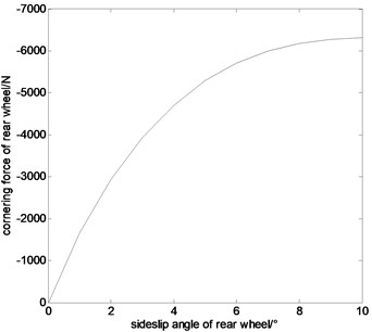
where $s_{1} ~ s_{7}$ are all identification parameters [14], and the values are $s_{1} = 777.88$ , $s_{2} = 0.39502$ , $s_{3} = 0.06075$ , $s_{4} = –0.0368$ , $s_{5} = 0.03755$ , $s_{6} = 1.0227$ , $s_{7} = 0.2289 8$ , $s_{8} = –0.2074 1$ .

Bringing the above parameters to the unified model and using the Matlab program, the relationship graphics between cornering force and sideslip angle of car’s front and rear wheels are shown in Fig. 1 and Fig. 2 respectively. Fig. 1 shows the relationship between cornering force and sideslip angle of front wheel. Fig. 2 shows the relationship between cornering force and sideslip angle of rear wheel.

From Fig. 1 and Fig. 2, when the sideslip angle is small, the relationship between cornering force and sideslip angle is linear. When the sideslip angle is large, the cornering force grows slowly. When the sideslip angle is 8 degree, the cornering force reaches saturation and almost stops growing.

Fig. 1The relationship between cornering force and sideslip angle of front wheel

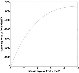
Fig. 2The relationship between cornering force and sideslip angle of front wheel

2.2. Full vehicle model

In the model, the vehicle travels at a constant speed $u$ , the inertia and damping of the steering system, the effect of suspension, the cornering properties change of left and right tires due to different vertical loads, and the influence of tire aligning torque are all ignored. As shown in Fig. 3, two generalized coordinates, yawing angle $ψ$ and centroid sideslip angle $β$ , are utilized to represent the vehicle’s motion state.

According to D’Alembert principle, the force equilibrium equations of the vehicle’s motion are as follows:

7

M u (ω_{r} + \dot{β}) = - (P_{y 1} + P_{y 2}),

8

I_{Z} {\dot{ω}}_{r} = - a P_{y 1} + b P_{y 2},

where, $I_{Z}$ is rotational inertia of the vehicle around $Z$ -axis and $P_{y 1}$ , $P_{y 2}$ are cornering force of front and rear wheels respectively.

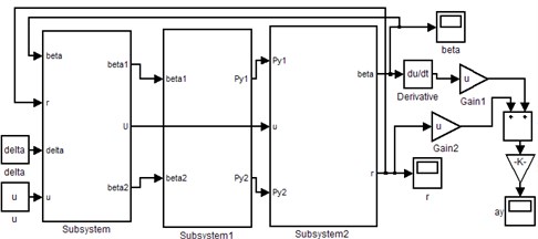
Considering nonlinear tire cornering properties and combining with vehicle dynamics equations, a two degrees of freedom (DOF) nonlinear vehicle steering motion model is built in Matlab/Simulink, as shown in Fig. 4.

Fig. 32DOF vehicle steering model

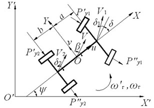
Fig. 42DOF nonlinear vehicle Simulink model

2.3. Experimental verification

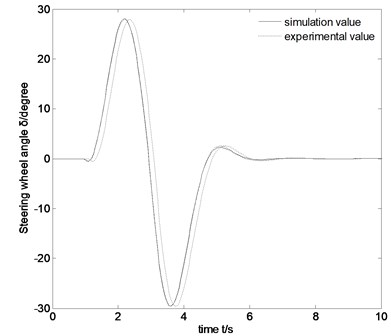
A single lane-change real vehicle test of a car is done in this paper, and the test data is collected to compare with the results of simulation test by using the above nonlinear vehicle steering motion model. Fig. 5 shows the comparison results.

As shown in Fig. 5, the tendency of the two curves is consistent, and the amplitude of the two curves is slightly different, but the total difference is in the allowable range and there is a little difference of time between the two curves. It shows that the nonlinear vehicle steering motion model conforms to the reality, so the results from the model are correct.

Fig. 5Comparison figure between a single lane-change test results and simulation results

3. Nonlinear vehicle steering control implementation

3.1. Basic theory

Single neuron self-adaptive PID control, which is based on quadratic form, is by means of quadratic performance index of optimal control in the single neuron learning algorithm index. Quadratic performance index is introduced into the adjustment of weighting coefficient. The weighting sum of squares for output error and controlled quantity is minimized to adjust weighting coefficient, in this way constrained control of output error and controlled increment is realized indirectly [15].

The performance index is supposed as follows:

9

J = \frac{1}{2} \{P {[r (k) - y (k)]}^{2} + Q [Δ^{2} (u (k))]\},

where, $P$ , $Q$ are weighting coefficient of output error and controlled increment respectively, $r (k)$ , $y (k)$ are reference input and output at the moment $k$ respectively, and $Δ u (k)$ is output increment of the controller.

The neurons output is:

10

u (k) = u (k - 1) + K [w_{P}^{'} (k) x_{P} (k) + w_{I}^{'} (k) x_{I} (k) + w_{D}^{'} (k) x_{P} (k)],

where, $b_{0}$ is the first value of the output response, and $w_{i} (k)$ is the weighted value corresponding to the neurons input, and $K$ is the proportion of neurons coefficient, and $K > 0$ .

11

\{\begin{matrix} w_{P}^{'} (k) = \frac{w_{P} (k)}{[|w_{P} (k)| + |w_{I} (k)| + |w_{D} (k)|]}, \\ w_{I}^{'} (k) = \frac{w_{I} (k)}{[|w_{P} (k)| + |w_{I} (k)| + |w_{D} (k)|]}, \\ w_{D}^{'} (k) = \frac{w_{D} (k)}{[|w_{P} (k)| + |w_{I} (k)| + |w_{D} (k)|]}, \end{matrix}

12

\{\begin{array}{l} x_{P} (k) = e (k) - e (k - 1), \\ x_{I} (k) = e (k), \\ x_{D} (k) = Δ^{2} e (k) = e (k) - 2 e (k - 1) + e (k - 2), \\ z (k) = e (k) . \end{array}

3.2. Vehicle steering control algorithm

At a constant speed, the driver’s desired trajectory of vehicle, in fact, is determined by the decision and track of the ideal lateral acceleration, and there is a one-to-one correspondence between the steering wheel angle changes and lateral acceleration changes. In this paper, two quadratic performance indexes, the trajectory following error and the busyness degree of steering wheel, are used to reflect vehicle handling stability, and their expressions are:

13

J_{1} = \frac{1}{2} {[{\ddot{y}}^{*} (k) - \ddot{y} (k)]}^{2},

14

J_{2} = \frac{1}{2} {[δ_{s w} (k) - δ_{s w} (k - 1)]}^{2} .

Therefore, the performance index function for vehicle steering single neuron controller is:

15

J = \frac{1}{2} \{P {[{\ddot{y}}^{*} (k) - y (k)]}^{2} + Q [δ_{s w} (k) - δ_{s w} (k - 1)]\},

where, ${\ddot{y}}^{*} (k)$ , $\ddot{y} (k)$ are the ideal lateral acceleration input and the actual lateral acceleration output at the moment $k$ respectively, $δ_{s w} (k)$ , $δ_{s w} (k - 1)$ are the steering wheel angle at the moment $k$ and $k - 1$ respectively, and $P$ , $Q$ are the weighting coefficient of the trajectory following error and the busyness degree of steering wheel.

Gradient descent method is a kind of iterative optimizing algorithms which is seeking the minimum of a particular performance index. Its basic idea is to make the correction of neurons’ connective weights $w_{i} (k)$ decrease along with direction of reduction of $J$ , that is:

16

Δ w_{i} (k - 1) = w_{i} (k) - w_{i} (k - 1) = - η_{i} \frac{\partial J}{\partial w_{i} (k - 1)} .

According to the established performance index function $J$ , gradient descent method is adopted to make optimizing design for the performance index function, which objective is to minimize $J$ , so as to realize the correction of neurons’ connective weights. The control rule and the learning algorithm of single neuron self-adaptive controller are as follows:

17

\{\begin{array}{l} e (k) = {\ddot{y}}^{*} (k) - \ddot{y} (k), \\ x_{P} (k) = e (k) - e (k - 1), \\ x_{I} (k) = e (k), \\ x_{D} (k) = Δ^{2} e (k) = e (k) - 2 e (k - 1) + e (k - 2), \end{array}

18

\{\begin{array}{l} T_{w x} (k - 1) = w_{I} (k - 1) x_{I} (k - 1) + w_{P} (k - 1) x_{P} (k - 1) + w_{D} (k - 1) x_{D} (k - 1), \\ w_{P} (k) = w_{P} (k - 1) + η_{P} K [P b_{0} e (k) x_{P} (k - 1) - Q K T_{w x} (k - 1) x_{P} (k - 1)], \\ w_{I} (k) = w_{I} (k - 1) + η_{I} K [P b_{0} e (k) x_{I} (k - 1) - Q K T_{w x} (k - 1) x_{I} (k - 1)], \\ w_{D} (k) = w_{D} (k - 1) + η_{D} K [P b_{0} e (k) x_{D} (k - 1) - Q K T_{w x} (k - 1) x_{D} (k - 1)], \end{array}

19

\{\begin{array}{l} {w'}_{P} (k) (k) = \frac{w_{P} (k)}{w_{I} (k) + w_{P} (k) + w_{D} (k)}, \\ w_{I}^{'} (k) = \frac{w_{I} (k)}{w_{I} (k) + w_{P} (k) + w_{D} (k)}, \\ w_{D}^{'} (k) = \frac{w_{D} (k)}{w_{I} (k) + w_{P} (k) + w_{D} (k)}, \end{array}

20

δ_{s w} (k) = δ_{s w} (k - 1) + K (w_{P}^{'} (k) x_{P} (k) + w_{P}^{'} (k) x_{I} (k) + w_{D}^{'} (k) x_{D} (k)),

where, $η_{P}$ , $η_{I}$ , $η_{D}$ are proportional, integral and differential learning rate respectively, $K$ is neuron proportion coefficient, and $b_{0}$ is the output response value of the control system at the initial state.

3.3. Vehicle steering control model

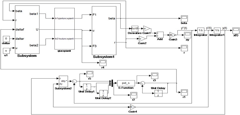
Transfer function cannot describe single neuron PID controller directly, and the simulation cannot be carried on by applying Matlab/Simulink simply, so the function $S$ is introduced to define the system dynamic characteristics, and pid_s module is built. A nonlinear 2DOF vehicle module and a single neuron self-adaptive PID module are connected to constitute the complete control system diagram, and computer simulation model is established by using Matlab/Simulink, as shown in Fig. 6. The control of the nonlinear 2DOF vehicle system by applying the single neuron self-adaptive control algorithm which is based on quadratic form is achieved, and precise tracking for single lane-change path comes true [16].

Fig. 6Computer simulation model

3.4. Simulation analysis

In order to simulate the vehicle emergency avoidance at high speed, driver’s preview-follower method which is aimed to determine the ideal lateral acceleration is directly used, and vehicle single lane-change condition (simulating emergency avoidance process) simulation calculation are conducted with 2DOF vehicle model which contains tire nonlinear cornering characteristics at different speeds from low to high. Meanwhile, in order to reflect the robustness of the algorithm while speed changes, proportional, integral and differential learning rate $η_{P}$ , $η_{I}$ , $η_{D}$ at different speeds. The neuron proportion coefficient $K$ , the weighting coefficient of the trajectory following error $P$ and the busyness degree of steering wheel $Q$ are all constant. Vehicle parameters are presented in Table 1.

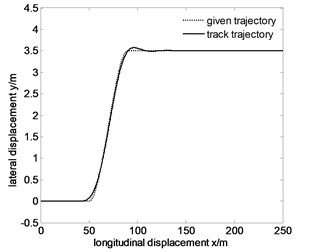
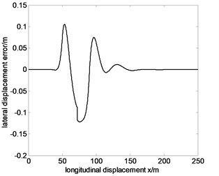
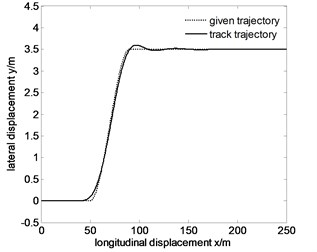
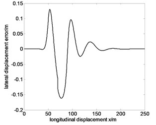
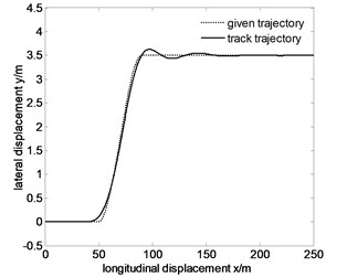
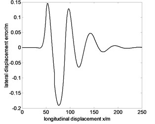
The situations of tracking the specified path at the speed $u = 60 km/h,$ $u = 80 km/h,$ $u = 100 km/h$ are presented in Fig. 7-9.

Table 1Parameters of vehicle

Parameter	Value
Vehicle mass ( $M$ )	1250 kg
Suspension mass ( $M_{s}$ )	900 kg
Front axle to CG ( $a$ )	1.170 m
Rear axle to CG ( $b$ )	1.195 m
Moment of inertia around $Z$ -axis ( $I_{z}$ )	1800 kg·m²
Effective cornering stiffness of front wheel ( $K_{f}$ )	–60042 N/rad
Effective cornering stiffness of rear wheel ( $K_{r}$ )	–60053 N/rad
Transmission ratio of steering system ( $i$ )	20

Fig. 7Tracking the specified path and lateral displacement error of 60 km/h before optimization

a)

b)

Fig. 8Tracking the specified path and lateral displacement error of 80 km/h before optimization

a)

b)

Fig. 9Tracking the specified path and lateral displacement error of 100 km/h before optimization

a)

b)

From Fig. 7-9, the maximum lateral displacement error at the speed of 60 km/h, 80 km/h and 100 km/h is about 0.1216 m, 0.1615 m and 0.1909 m, respectively. On the whole, the vehicle tracks the given trajectory well, which proves that the vehicle has good steering handling trajectory following performance, and single neuron PID control has stronger robustness and adaptability for speed changes. But with the increase of speed, trajectory following error also increases. The main reasons are the following two points.

(1) While emphasizing tracking accuracy, the trajectory following error and the busyness degree of steering wheel are considered comprehensively.

(2) With the increase of speed, the nonlinear characteristics of vehicle become more obvious, but the precision of the single neuron self-adaptive control algorithm declines slightly.

4. Nonlinear vehicle steering control optimization

4.1. Multi-island genetic algorithm

In this paper, control parameter optimizing design through multi-island genetic algorithm is used to realize the optimal control of the control system [14]. Multi-island genetic algorithm is a kind of pseudo parallel genetic algorithm. Compared with traditional genetic algorithms, it divides the whole evolution population into several subgroups which are called “islands”. Then “migration” operation to subgroups in every island is done, which transfers those subgroupsto other islands. The above measure can keep the diversity of population, so the precocious phenomenon of evolution is suppressed. The optimizing procedures are as follows:

(1) Determine the optimal design variables, and then establish the optimizing model.

(2) Determine the coding method, genetic control parameters, population’s size, terminal conditions, and fitness function.

(3) Initialize the population, and conduct fitness evaluation.

(4) Judge whether the terminal conditions meet the requirements, if meet, output optimal results, otherwise, turn to step (5) and conduct genetic operations to create new species.

(5) Genetic operations, according to the previous genetic control parameters, are that selecting individuals randomly to do crossover and mutation operations in sub populations. Then optimal save operation for the previous generation’s optimal individual will be done, and finally produce the next generation.

4.2. Simulation analysis

Based on the “inverse problem” solving, the optimizing model is:

21

\min J,

22

s.t. {\underline{b}}_{i} \leq b_{i} \leq {\bar{b}}_{i}, (i = 1,2, \dots, 6)

where, $b_{i}$ is the control parameter.

In the process of optimization, some high speed evaluation indexes need to be punished, so a punishing item $1 + {(T_{c} / {\hat{T}}_{c})}^{2} + {(T u / \hat{D})}^{4}$ is added. The vehicle handling performance evaluation index takes the following form:

23

J = \frac{1}{2} [1 + {(T_{c} / {\hat{T}}_{c})}^{2} + {(T u / \hat{D})}^{4}] \cdot \{P {[{\ddot{y}}^{*} (k) - y (k)]}^{2} + Q {[δ_{s w} (k) - δ_{s w} (k - 1)]}^{2}\} .

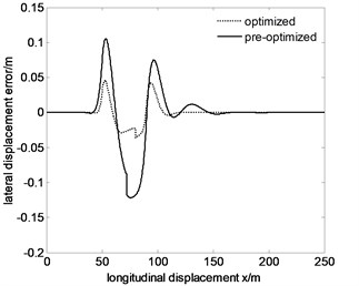
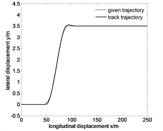
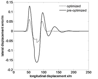
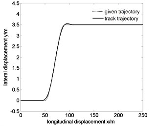
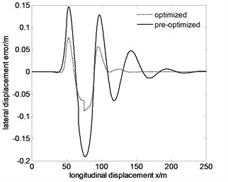
In the optimizing process, for every set of optimized parameter values, a given track is followed. After optimization by using genetic algorithm, the situation of tracking the specified path at the speed of $u = 60 km/h,$ $u = 80 km/h,$ $u = 100 km/h,$ and path tracking error comparison before and after optimization are shown in Fig. 10-12.

From Fig. 10 to Fig. 12, maximum lateral displacement error at the speed $u = 60 km/h$ , $u = 80 km/h$ , $u = 100 km/h$ are 0.0454 m, 0.0610 m, 0.0878 m respectively. Comparing the above values with the pre-optimized values 0.1216 m, 0.1615 m, 0.1909 m, they reduce significantly. To ensure the maneuverability of the vehicle, the comparison between the optimized Fig. 10-12 and the pre-optimized Fig. 10-12 show that the trajectory error decreases, so the tracking accuracy improves.

Fig. 10Tracking the specified path and lateral displacement error of 60 km/h after optimization

a)

b)

Fig. 11Tracking the specified path and lateral displacement error of 80 km/h after optimization

a)

b)

Fig. 12Tracking the specified path and lateral displacement error of 100 km/h after optimization

a)

b)

5. Conclusions

(1) Aiming at the present situation of less research on nonlinear vehicle high-speed emergency avoidance, tire nonlinear cornering model is established and the validity of the model is verified by the real vehicle test in this paper. On the basis of the above mentioned research, avoidance conditions for a single lane change is set and single neuron self-adaptive PID algorithm is put forward which is based on quadratic form. Through the above measures, the trajectory tracking is realized, and the relatively accurate control performance is reflected, as well as robustness and adaptability to the change of speed.

(2) In accordance with related theories, this paper applies multi-island genetic algorithm to optimize single neuron PID control algorithm, and the results show that the method can improve the accuracy of path tracking effectively at different speeds. The research not only proves the feasibility of genetic algorithm in the study of nonlinear vehicle high-speed emergency avoidance, but also shows that the measure in this paper has certain reference value to the problem of auxiliary driving.

References

Mas A., Merienne F., Kemeny A. Lateral control assistance and driver behavior in emergency situations. Advances in Transportation Studies, Special, 2011, p. 149-158.

Search CrossRef
Hattori Y., Ono E., Hosoe S. Optimum vehicle trajectory control for obstacle avoidance problem. IEEE/ASME Transactions on Mechatronics, Vol. 11, Issue 5, 2006, p. 507-512.

Search CrossRef
Kurzhanski A. B. Dynamic optimization for nonlinear target control synthesis. The 6th IFAC Symposium on Nonlinear Control Systems, Stuttgart, Germany, 2004, p. 20-34.

Search CrossRef
Richards A., How J. Aircraft trajectory planning with collision avoidance using mixed integer linear programming. American Control Conference, Anchorage, AK, USA, 2002, p. 1936-1941.

Search CrossRef
Ryu J., Kim H. S., Kim J. H. An emergency obstacle avoidance control strategy for automated highway vehicles. Vehicle System Dynamics, Vol. 38, Issue 5, 2002, p. 319-339.

Search CrossRef
Hagenaars H., Imura J., Nijmeijer H. Approximate continuous-time optimal control in obstacle avoidance by time/space discretization of non-convex state constrains. IEEE Conference on Control Applications, Taipei, Taiwan, China, 2004, p. 878-883.

Search CrossRef
Mukai M., Kawabe T., Nishira H., Takagi Y., Deguchi Y. On vehicle path generation method for collision avoidance using mixed integer programming. The 16th IEEE International Conference on Control Applications Part of IEEE Multi-conference on Systems and Control, Singapore, 2007, p. 1371-1374.

Search CrossRef
Darguzis A., Sapragonas J., Pilkauskas K. Dynamic processes of a vehicle moving over step-shaped obstacles. Journal of Vibroengineering, Vol. 13, Issue 3, 2011, p. 536-343.

Search CrossRef
Ghaffari A., Khodayari A., Arvin S., Alimardani F., Lagnemma K. An ANFIS design for prediction of future state of a vehicle in lane change behavior. IEEE International Conference on Control System, Computing and Engineering, Penang, Malaysia, 2011, p. 156-161.

Search CrossRef
Jin S., Huang Z., Tao P., Wang D. Car-following theory of steady-state traffic flow using time-to-collision. Journal of Zhejiang University-Science A, Applied Physics & Engineering, Vol. 12, Issue 8, 2011, p. 645-654.

Search CrossRef
Konghui G., Ye Z., Dang L. A study on speed-dependent tyre-road friction and its effect on the force and the moment. Vehicle System Dynamics, Vol. 43, 2005, p. 329-340.

Search CrossRef
Konghui G., Dang L., ShiKen C. The unitire model: a nonlinear and non-steady-state tyre model for vehicle dynamics simulation. Vehicle System Dynamics, Vol. 43, 2005, p. 341-358.

Search CrossRef
Konghui G., Nan X., Dang L. A model for combined tire cornering and braking forces with anisotropic tread and carcass stiffness. SAE International Journal of Commercial Vehicles, Vol. 4, Issue 1, 2011, p. 84-95.

Search CrossRef
Umsrithong A., Sandu C. Stochastic transient tyre model for vehicle dynamic simulations on rough rigid ground. International Journal of Vehicle Systems Modeling and Testing, Vol. 7, Issue 4, 2012, p. 351-371.

Search CrossRef
Wang W., Zhou J., Fan, Y. Parameters optimization of laser shot peening based on multi-island genetic algorithm. Applied Mechanics and Materials, Vol. 43, 2011, p. 387-390.

Search CrossRef
Hanxu S., Hou K., Qingxuan J. Development, analysis and control of a spherical aerial vehicle. Journal of Vibroengineering, Vol. 15, Issue 2, 2013, p. 1069-1080.

Search CrossRef

About this article

Received

25 September 2013

Accepted

21 December 2013

Published

31 March 2014

Keywords

genetic algorithm

nonlinear

emergency avoidance

steering control

parameter optimization

Acknowledgements

This work was supported in part by the National Science Foundation of China (Grant No. 11072106).

This is an open access article distributed under the Creative Commons Attribution License, which permits unrestricted use, distribution, and reproduction in any medium, provided the original work is properly cited.