A spectral method to estimate fatigue life under broadband non-Gaussian random vibration loading

Cheng, Hongwei; Tao, Junyong; Chen, Xun; Jiang, Yu

Journal of Vibroengineering

Browse Journal

Submit article

Published: 31 March 2014

Check for updates

A spectral method to estimate fatigue life under broadband non-Gaussian random vibration loading

Hongwei Cheng¹

Junyong Tao²

Xun Chen³

Yu Jiang⁴

^{1, 2, 3, 4}Science and Technology on Integrated Logistics Support Laboratory National University of Defense Technology, 410073, P. R. China

^{1, 2, 3, 4}College of Mechatronic Engineering and Automation National University of Defense Technology, 410073, P. R. China

Corresponding Author:

Junyong Tao

Cite the article Download PDF

Downloads 1748

WoS Core Citations 4

Abstract

The aim of this study is to propose a spectral method for assessing the fatigue lives of mechanical components under non-Gaussian random vibration loadings. Efforts are made to extend the Dirlik’s method to non-Gaussian vibration field by introducing the Gaussian mixture model. A symmetric non-Gaussian random vibration can be decomposed into a series of Gaussian components through Gaussian mixture model. Then the rainflow cycle distributions of the Gaussian components can be obtained using Dirlik’s method. The cycle distribution of the underlying non-Gaussian process is derived by compounding the distributions of Gaussian components together. The non-Gaussian cycle distribution, combined with Palmgren-Miner rule is used to predict the fatigue lives of specimens. Comparisons among the proposed method, Dirlik’s solution, nonlinear model in literature, and the experimental data, are carried out extensively. The results have confirmed good accuracy of the proposed method.

1. Introduction

For some mechanical components, the service loadings are induced by random vibrations. The randomness of stress-time histories makes the assessment of fatigue damage quite difficult. Among all the cycle counting methods, the rainflow method is regarded as the best one [1]. In the time domain, the rainflow method is applicable for any kind of random process, but it usually requires a large amount of loading records from lengthy and expensive experimental data acquisition programs [2]. Furthermore, we cannot get a stable distribution of rainflow cycles from the time domain data [3]. The frequency-domain representations of random processes, normally power spectral densities (PSDs), are easier to apply and more flexible in engineering applications.

For spectral methods, the rainflow cycle distributions are usually estimated based on the PSDs. Based on Gaussian assumption some spectral methods have been proposed in the literature, such as narrow-band approximation method [4], Dirlik’s solution [5] and the methods presented in [6, 7]. A comparison of several spectral methods was presented in [8], where the precision of Dirlik’s method was validated.

In many cases, however, the dynamic vibration loadings of mechanical components do not follow Gaussian distributions [9-11]. The non-Gaussian nature of the stress response results from non-Gaussian external excitation, nonlinearity, or both [2]. The non-Gaussian random vibration loadings can accelerate the fatigue-damage accumulation because of the presence of high-excursion loading cycles. Hence, the spectral methods applicable to Gaussian loadings are not useful in non-Gaussian case. The methods based on Gaussian assumption will overestimate the fatigue lives of mechanical components subjected to non-Gaussian random loadings, possibly leading to serious accidents. Hence, new method which is effective for non-Gaussian stress-time histories is required.

Some spectral methods for non-Gaussian random loadings have been presented in literature. A narrow-band approximation method modified by non-normality and bandwidth correction coefficients was presented in [12]. Some methods based on nonlinear transformations of Gaussian processes were proposed in [2, 10, 13]. There are many damage accumulation rules proposed in the past. Generally speaking, the Palmgren-Miner rule [14, 15] could provide reliable fatigue damage estimation for stationary random loadings [2, 6].

Although some spectral methods for stationary non-Gaussian loadings have been proposed, simpler and more efficient methods are still needed in engineering practice. The method proposed in this paper is based on Dirlik’s formula. On the basis of the mathematical treatment of Gaussian mixture models (GMMs) for non-Gaussian noise in telecommunications applications [16, 17], a Gaussian mixture model is proposed here which is available for symmetric non-Gaussian loadings whose skewness values are zero and kurtosis values are three. Using the proposed Gaussian mixture model, a non-Gaussian loading can be decomposed into a series of Gaussian components with different probability weighting factors. Then Dirlik’s formula is used to obtain the cycle distributions of the Gaussian components. The cycle distribution of the non-Gaussian loading is obtained by compounding the distributions of the components with the proposed Gaussian mixture model. The non-Gaussian cycle distribution, combined with Palmgren-Miner rule is used to predict the fatigue lives of test specimens. Comparisons among the proposed method, nonlinear model in [18], Dirlik’s solution, and the experimental data, are carried out extensively. The results have confirmed good accuracy of the proposed method.

2. Non-Gaussian random vibration loadings

This study focuses on symmetrical non-Gaussian random loadings. Non-Gaussian vibrations are widely present in real-world environments. Theoretically, the statistical parameters that can thoroughly represent a non-Gaussian process are higher-order statistics: higher-order moments or higher-order cumulants [19]. The higher-order statistics of a random process are functions of the sequence of time lags ${τ_{i}}$ , $i = 1, 2, \dots, n$ . The estimation of higher-order statistics is a highly complex problem. In vibration engineering, the higher-order statistics by setting the time lags ${τ_{i}}$ to be zero are always used as substitutions. For this reason, certain statistical properties of the non-Gaussian random processes are ignored. This means that most spectral methods for non-Gaussian loadings are empirical or semi-empirical solutions. The most commonly used statistics are the normalized third- and fourth-order central moments: skewness ( $γ_{3}$ ) and kurtosis ( $γ_{4}$ ). Denoting by $X (t)$ a non-Gaussian random loading, skewness and kurtosis are defined as follows:

1

γ_{3} = \frac{E [{(X - μ_{X})}^{3}]}{σ_{X}^{3}} = \frac{m_{3}}{σ_{X}^{3}}, γ_{4} = \frac{E [{(X - μ_{X})}^{4}]}{σ_{X}^{4}} = \frac{m_{4}}{σ_{X}^{4}},

where $E [\cdot]$ denotes mathematical expectation, $μ_{X}$ and $σ_{X}$ are the mean value and the standard deviation of $X (t)$ and $m_{3}$ and $m_{4}$ are the third- and fourth-order central moments. In fact, skewness and kurtosis cannot represent the non-normality of a non-Gaussian process completely because the statistics higher than fourth-order are ignored and the properties of temporal correlation are neglected. It is not difficult to imagine a case that two different stationary non-Gaussian processes having identical variance, skewness, and kurtosis. In engineering filed, however, some simplifications are unavoidable. For Gaussian processes, the skewness and kurtosis values are zero and three respectively.

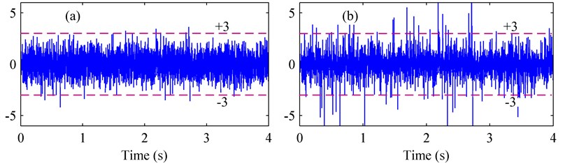
The non-Gaussian properties of vehicular vibrations are investigated in [11, 20], where it has been pointed out that most of the non-Gaussian loadings encountered in engineering practice are non-stationary from a short-duration viewpoint, but stationary from a longer-duration viewpoint. In engineering practice, these kinds of loadings are always treated as stationary processes for simplicity. This study is also partially based on this assumption. A comparison between standardized Gaussian and non-Gaussian processes is shown in Fig. 1. The discrepancy is prominent, and the non-Gaussian process has many higher-excursion peaks.

Fig. 1The standardized Gaussian and non-Gaussian processes: (a) Gaussian, (b) non-Gaussian (γ4= 8)

3. Gaussian mixture model (GMM)

In the study of non-Gaussian noise models in signal processing, Middleton proposed the Gaussian mixture model [16]. From the viewpoint of this model, the underlying non-Gaussian process consists of a series of Gaussian components, with different probability weight factors and other parameters. The original GMM was proposed mainly for estimating the non-Gaussian noise probability density function (PDF) in telecommunications applications. The general form of the GMM is:

2

f_{N G} (x) = \sum_{i = 1}^{N} α_{i} f_{i} (x),

where $f_{N G} (x)$ is the PDF of the non-Gaussian process; $f_{i} (x)$ is the Gaussian term, namely the PDF of the $i$ th Gaussian component; $α_{i}$ is the probability weighting factor, 0 ≤ $α_{i}$ ≤ 1, $\sum α_{i} = 1$ ; and $N$ is the dimension of GMM.

For the original GMM in telecommunications applications, the weighting factor $α_{i}$ is quantified by a Poisson distribution based on thorough understanding of each Gaussian noise source. This is impossible for non-Gaussian random loadings in mechanical engineering. Hence, a modified GMM is needed which is available for non-Gaussian random loadings.

Normally, a rather small value of $N$ in Eq. (2), is sufficient to provide an excellent approximation of the real distribution function [17]. The two-term GMM will be used here:

3

f_{N G} (x) = α f_{1} (x) + (1 - α) f_{2} (x) .

For a zero-mean stationary non-Gaussian process $X (t)$ , the GMM can be expressed as:

4

f_{N G} (x) = α \frac{1}{\sqrt{2 π} σ_{1}} e x p (- \frac{x^{2}}{2 σ_{1}^{2}}) + (1 - α) \frac{1}{\sqrt{2 π} σ_{2}} e x p (- \frac{x^{2}}{2 σ_{2}^{2}}),

where $σ_{1}$ and $σ_{2}$ are the standard deviations of the two Gaussian components and $α$ and ( $1 - α$ ) are the probability weighting factors of the two terms. There are three unknown quantities $σ_{1}$ , $σ_{2}$ , and $α$ , in Eq. (4). Therefore, a three-variable set of equations is needed to derive the unknown parameters.

For real non-Gaussian random loadings in engineering practice, the true values of the higher-order moments cannot be known. The estimated values are always used as substitutes. For a zero-mean process, the second-, fourth-, and sixth-order moments can be calculated as follows:

5

\{\begin{array}{l} m_{2} = E [x^{2}] = \int_{- \infty}^{\infty} x^{2} f_{N G} (x) d x ≅ {\hat{m}}_{2} = \frac{1}{T} \int_{0}^{T} x^{2} (t) d t, \\ m_{4} = E [x^{4}] = \int_{- \infty}^{\infty} x^{4} f_{N G} (x) d x ≅ {\hat{m}}_{4} = \frac{1}{T} \int_{0}^{T} x^{4} (t) d t, \\ m_{6} = E [x^{6}] = \int_{- \infty}^{\infty} x^{6} f_{N G} (x) d x ≅ {\hat{m}}_{4} = \frac{1}{T} \int_{0}^{T} x^{6} (t) d t, \end{array}

where $T$ is the duration of the sample time history. When $T$ is long enough, these estimates will converge to the true values with sufficient precision [21].

By substituting Eq. (4) into Eq. (5), the following equations can be obtained:

6

\{\begin{array}{l} m_{2} = α m_{2}^{(1)} + (1 - α) m_{2}^{(2)}, \\ m_{4} = α m_{4}^{(1)} + (1 - α) m_{4}^{(2)}, \\ m_{6} = α m_{6}^{(1)} + (1 - α) m_{6}^{(2)}, \end{array}

where $m_{2}^{(1)}$ and $m_{2}^{(2)}$ are the second-order moments of the two Gaussian components, $m_{4}^{(1)}$ and $m_{4}^{(2)}$ are the fourth-order moments, and $m_{6}^{(1)}$ and $m_{6}^{(2)}$ are the sixth-order moments. The second-order moments are equal to the variances, $σ_{1}^{2}$ and $σ_{2}^{2}$ .

For a zero-mean stationary Gaussian process, the following relationship exists between the various ordered moments:

7

m_{k} = \{\begin{array}{l} [1 \times 3 \times 5 \dots (k - 1)] σ^{k}, & k is   even, \\ 0, & k is   odd, \end{array}

where $σ$ is the standard deviation or root mean square (RMS) and $k$ is a positive integer, 1 ≤ $k$ < $\infty$ . Then for the two Gaussian components:

8

\{\begin{array}{l} m_{2}^{(1)} = σ_{1}^{2}, & m_{2}^{(2)} = σ_{2}^{2}, \\ m_{4}^{(1)} = 3 σ_{1}^{4}, & m_{4}^{(2)} = 3 σ_{2}^{4}, \\ m_{6}^{(1)} = 15 σ_{1}^{6}, & m_{6}^{(2)} = 15 σ_{2}^{6} . \end{array}

Substituting Eq. (8) into Eq. (6) results in:

9

\{\begin{array}{l} m_{2} = α σ_{1}^{2} + (1 - α) σ_{2}^{2}, \\ m_{4} = 3 α σ_{1}^{4} + 3 (1 - α) σ_{2}^{4} \\ m_{6} = 15 α σ_{1}^{6} + 15 (1 - α) σ_{2}^{6} . \end{array}

The unknown parameters $σ_{1}$ , $σ_{2}$ , and $α$ can be derived through Eq. (9) by substituting the theoretical values of $m_{1}$ , $m_{2}$ , and $m_{3}$ by the estimated ones in Eq. (5). Then the two-term mixture PDF of a non-Gaussian process is obtained. This is a new method for estimating the PDFs of symmetric non-Gaussian loadings. However, to assess the fatigue cycle distribution of non-Gaussian random loadings based on spectral data, a further step must be taken. Hence, the GMM will be introduced into the frequency domain.

4. PSD decomposition of non-Gaussian vibration loadings

It is clear that a PSD cannot define a non-Gaussian process, unlike the Gaussian case. Based on the GMM, a probabilistic explanation of a non-Gaussian process has been proposed. In Eq. (4), $α$ and ( $1 - α$ ) represent the probabilities of existence of the two Gaussian components in the time domain. Furthermore, in the frequency domain, the underlying PSD is decomposed into two different-valued PSDs to account for non-normality.

For a non-Gaussian zero-mean stationary process $X (t)$ , the variance can be expressed as:

10

σ_{X}^{2} = \int_{0}^{\infty} S_{X} (f) d f,

where $S_{X} (f)$ is the one-sided PSD, and $f$ is the frequency. For the two Gaussian components:

11

σ_{1}^{2} = \int_{0}^{\infty} S_{1} (f) d f, σ_{2}^{2} = \int_{0}^{\infty} S_{2} (f) d f,

where $S_{1} (f)$ and $S_{2} (f)$ are the PSDs of the two components. According to Eq. (9):

12

σ_{X}^{2} = α σ_{1}^{2} + (1 - α) σ_{2}^{2} .

Substituting Eq. (10) and Eq. (11) into Eq. (12), results in:

13

S_{X} (f) = α S_{1} (f) + (1 - α) S_{2} (f) .

To derive the PSD-based rainflow cycle distribution, the magnitudes of $S_{1} (f)$ and $S_{2} (f)$ must be determined. Here we assume that $S_{1} (f)$ and $S_{2} (f)$ are proportional to $S_{X} (f)$ along the frequency axis:

14

S_{1} (f) = η_{1} S_{X} (f), S_{2} (f) = η_{2} S_{X} (f),

where $η_{1}$ and $η_{2}$ are the constants of proportionality, which can be derived by combining Eq. (14) with Eq. (10) and Eq. (11):

15

η_{1} = \frac{σ_{1}^{2}}{σ_{X}^{2}}, η_{2} = \frac{σ_{2}^{2}}{σ_{X}^{2}} .

Then, substituting Eq. (14) and Eq. (15) into Eq. (13), the PSD decomposition of symmetric non-Gaussian random loadings is obtained. The expression in Eq. (13) is defined as the probabilistic PSD ( $p$ -PSD).

5. Modified Dirlik’s formula and fatigue damage estimation

5.1. Dirlik’s formula

Dirlik’s formula is an approximate closed-form expression of the PDF of the normalized amplitude of rainflow cycles. This method has been developed based on extensive numerical simulations with computers [5]. First, let us introduce the definition of spectral moment. For the PSD of a given Gaussian process $X (t)$ , the spectral moment is defined as:

16

λ_{n} = \int_{0}^{\infty} f^{n} S_{X} (f) d f .

From spectral moments, it is possible to derive some important characteristics of the random process itself. For example, the standard deviation is $σ_{X} = \sqrt{λ_{0}},$ the expected rate of zero-uncrossing is $v_{0} = \sqrt{λ_{2} / λ_{0}}$ , the expected rate of peaks is $v_{p} = \sqrt{λ_{4} / λ_{2}}$ , the bandwidth factor is $B = v_{0} / v_{p}$ , and the average frequency is $f_{m} = λ_{1} / λ_{0} \sqrt{λ_{2} / λ_{4}}$ .

The normalized amplitude of the loading cycle is defined as:

17

z = s / σ_{X},

where $s$ is the amplitude of the rainflow cycle. Then the distribution of the normalized rainflow cycle, based on Dirlik’s solutions, is [5]:

18

p (z) = c_{1} \frac{1}{ϖ} e x p (- \frac{z}{ϖ}) + c_{2} \frac{z}{ξ^{2}} e x p (- \frac{z^{2}}{2 ξ^{2}}) + c_{3} z e x p (- \frac{z^{2}}{2}),

where $c_{1} = \frac{2 (f_{m} - B^{2})}{1 + B^{2}},$ $c_{2} = \frac{1 - B - c_{1} + c_{1}^{2}}{1 - ξ},$ $c_{3} = 1 - c_{1} - c_{2},$ $ϖ = \frac{1.25 (B - c_{3} - c_{2} ξ)}{c_{1}},$ $ξ = \frac{B - f_{m} - c_{1}^{2}}{1 - B - c_{1} + c_{1}^{2}}$ . Previous studies have proved that Dirlik’s empirical formula can precisely approximate the rainflow cycle distributions of Gaussian random loadings [8].

5.2. Dirlik’s formula for non-Gaussian loadings

Equation (13) gives the $p$ -PSD of a non-Gaussian random loading. Then the rainflow cycle distribution of each component can be calculated based on Dirlik’s formula through a simple variable change:

19

p_{1} (s) = {\frac{p_{1} (z)}{σ_{1}}|}_{z = \frac{s}{σ_{1}}}, p_{2} (s) = {\frac{p_{2} (z)}{σ_{2}}|}_{z = s / σ_{2}},

where $p_{1} (z)$ and $p_{2} (z)$ are the normalized cycle distributions of the Gaussian components, $s$ is the amplitude of the rainflow cycle, and $σ_{1}$ and $σ_{2}$ are the standard deviations of the two Gaussian components. The cycle distribution of the symmetric non-Gaussian random loading is defined as follows:

20

f_{G M M} (s) = α p_{1} (s) + (1 - α) p_{2} (s) .

5.3. Fatigue damage estimation

For a random loading, fatigue damage is caused by amplitudes and mean values of loading cycles. The counted cycles are random events. For zero mean non-Gaussian random loadings, the rainflow cycles follow the distribution expressed by Eq. 20. For nonzero mean loadings, the rainflow cycle distribution should be modified based on the correction models, such as Goodman model, Gerber model, and Soderberg model [22].The expected rate of occurrence of rainflow cycles is denoted with $v_{c}$ which is equal to the expected rate of occurrence of peak, $v_{p}$ . It is can be derived from the spectral moments of PSD, as shown in subsection 5.1.

Furthermore, a damage accumulation rule must be selected to collect the fatigue damage caused by each cycle together in a specified manner. There are many damage accumulation rules reviewed in [23]. The linear damage accumulation rule, namely Palmgren-Miner rule can give reasonable results for stationary random loadings according to [24]. We will adopt Palmgren-Miner rule in this study. Normally, the stress life curve, namely S-N curve is defined in the form of power-low model:

21

N S^{b} = A,

where, $N$ is the number of cycles to failure at amplitude $S$ , $b$ and $A$ are the fatigue parameters of material or structure. Then the expected fatigue damage can be expressed as follows:

22

E [D_{N G}] = \frac{v_{c} T}{A} \int_{0}^{\infty} s^{b} f_{G M M} (s) d s,

where $T$ is the time duration of the non-Gaussian random loading, $f_{G M M} (s)$ is the non-Gaussian rainflow cycle distribution defined in Eq. (20).

6. Examples

The fatigue data used in the examples is from Kihl [18]. This fatigue data and the simulated non-Gaussian random loadings are used to validate the capability of the proposed method. The proposed method is used to predict the fatigue lives of the fatigue test specimens (Fig. 2). Comparisons among experimental data, results from the proposed method, nonlinear transformation model, and Gaussian assumption are carried out extensively. In addition, a rainflow counting procedure based on the time history is carried out to evaluate the empirical distribution of rainflow cycles. The rainflow counting procedure is based mainly on the WAFO toolbox [25].

Fig. 2Fatigue test specimen [18] (Dimensions are in millimeters)

The cruciform joint shown in Fig. 2 was extensively tested under non-Gaussian random loadings. The welds in the specimens are common locations for initiation and propagation of fatigue cracks in actual structures. The configuration and dimensions of the test specimens are shown in Fig. 2. The yield stress and ultimate stress of the steel palate are 638 and 683 MPa, respectively. During the fatigue tests, the cruciforms were loaded axially in the vertical direction with loads applied to the ends of the vertical legs by means of hydraulic grips. Owing to the presence of stress concentrations and residual stresses at the weld toe, the fatigue cracks normally began at the toe of the welds, as shown in Fig. 2. The S-N curve of the structural detail is:

23

N S^{3.210} = 1.7811 \times 10^{12} .

The expression in Eq. (23) was fitted based on the results of constant-amplitude fatigue tests in four different stress levels where the lowest and highest levels are 83 and 310 MPa, respectively.

The non-Gaussian random loadings are generated using the standard Gaussian simulation technique [26] combined with nonlinear transformation [18]. The kurtosis value of the non-Gaussian loadings is five. The three RMS stress levels used in the experiments are 52, 69 and 103 MPa. The sample time histories and the PSDs of the broadband non-Gaussian random loadings in different RMS stress levels are shown in Fig. 3.

Fig. 3Sample time histories and the PSDs of the three broadband non-Gaussian random loadings in different RMS stress levels: (a) 52 MPa, (b) 69 MPa, (c) 103 MPa and (d) PSDs

Sample time histories and the PSDs of the three broadband non-Gaussian random loadings in different RMS stress levels: (a) 52 MPa, (b) 69 MPa, (c) 103 MPa and (d) PSDs

Each simulated load was used as input in the fatigue test and, treated as a loading block, was repeated many times until failure [18]. Four specimens were tested for each loading process. The broadband non-Gaussian fatigue test results are shown in Table 1. Also presented in this table are the mean values of fatigue lives, in applied cycles, for each stress level.

Table 1Broadband non-Gaussian fatigue test results

RMS stress level (MPa)	Cycle to failure, $N_{e x p}$
RMS stress level (MPa)	Exp. 1	Exp. 2	Exp. 3	Exp. 4	Mean value, ${\bar{N}}_{e x p}$
52	951800	742900	1067900	703000	866400
69	373800	326300	273000	301000	318525
103	47900	45100	39500	44200	44175

The critical fatigue damage is assumed to be $D_{c r} = 1$ , and then the predicted number of cycles to failure based on the proposed method (Eq. (22)) is:

24

N_{G M M} = v_{c} T = \frac{A}{\int_{0}^{\infty} s^{b} f_{G M M} (s) d s} .

In this example, $A =$ 1.7811×10¹², $b =$ 3.210. The rainflow cycle distribution $f_{G M M} (s)$ is derived based on the proposed method. For simplicity, we shall just demonstrate the application of the proposed method to the case that the RMS stress level is 52 MPa. The procedures for other cases are similar, and we will just list the results.

Based on Eq. (5), we get the estimations of the second-, fourth-, and sixth-order moments of the non-Gaussian random loading shown in Fig. 3(a), ${\hat{m}}_{2} =$ 2704, ${\hat{m}}_{4} =$ 3.8564×10⁷, and ${\hat{m}}_{6} =$ 1.2044×10¹². By substituting these values into Eq. (9), we get the parameters of GMM are, $α =$ 0.7560, $σ_{1} =$ 36.9662, and $σ_{2} =$ 82.7539. And then according to Eq. (15), the two parameters for $p$ -PSD are:

25

η_{1} = \frac{σ_{1}^{2}}{σ_{X}^{2}} = {(\frac{36.9662}{52})}^{2} = 0.5054, η_{2} = \frac{σ_{2}^{2}}{σ_{X}^{2}} = {(\frac{82.7539}{52})}^{2} = 2.5326.

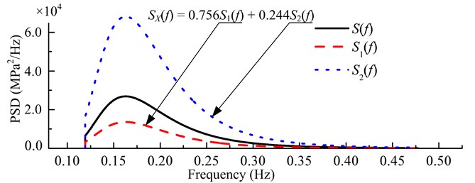
Based on these two parameters and Eq. (13), the $p$ -PSD of the non-Gaussian loading is obtained, as shown in Fig. 4.

Fig. 4p-PSD of the non-Gaussian random loading with RMS stress level 52 MPa

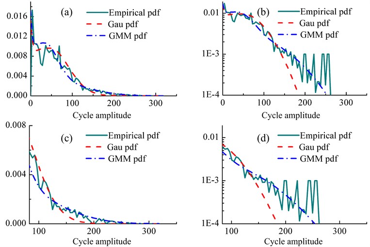
By substituting $S_{1} (f)$ and $S_{2} (f)$ into the Dirlik formula (Eq. (18) and Eq. (19)), we can get two Gaussian rainflow cycle distributions, $p_{1} (s)$ and $p_{2} (s)$ . And then we can get the non-Gaussian rainflow cycle distribution according to Eq. (20), as shown in Fig. 5. Also illustrated in this figure are the empirical distribution and Gaussian rainflow cycle distribution. The empirical distribution is estimated based on rainflow cycles counted from the sample time history with time duration $T =$ 4000 s. There are 1425 rainflow cycles in the sample time history. The comparison shows the accuracy of the proposed in describing the rainflow cycle distribution of broadband non-Gaussian random loading. The full range comparisons are presented in Fig. 5(a) and Fig. 5(b) in the linear and semi-log coordinates, respectively. And we can see that the proposed methodology can give a reasonable description of the non-Gaussian rainflow cycle distribution, especially in the larger range of the rainflow cycles. Normally, the larger cycles will dominate the fatigue damage process of mechanical component, so we have given a close up view of the distribution curves when cycle amplitude is above 83 MPa in both linear and semi-log scales in Fig. 5(c) and Fig. 5(d), respectively. Furthermore, we can see that the empirical distribution curve fluctuates severely when the PDF value is close to or below 0.1 % in semi-log scale. The reason for this phenomenon is that the sample size of the rainflow cycles is 1425, which is too small to give a stable prediction in that order of magnitude. But the proposed method can give a stable prediction, as shown in Fig. 5(b) and (d).

The predicted fatigue life of the specimen is derived by substituting the non-Gaussian rainflow cycle distribution into Eq. (24). The mean values of the test fatigue data together with the predicted results based on the proposed method (Eq. (24)), the nonlinear transformation model in [18], and Dirlik formula, in three RMS stress levels are shown in Table 2, where:

${\bar{N}}_{e x p}$ indicates the mean values of fatigue data in Table 1,

$N_{G M M}$ indicates the results from the proposed method,

$N_{K i h l}$ indicates the results from the nonlinear transformation model [18],

$N_{G}$ indicates the results based on Gaussian assumption, namely Dirlik solution.

Table 2Comparison of fatigue lives for broadband non-Gaussian loadings (γ4= 5)

RMS stress level (MPa)	Cycles to failure
RMS stress level (MPa)	${\bar{N}}_{e x p}$	$N_{G M M}$		$N_{K i h l}$		$N_{G}$
52	866400	891600	(2.91 %)	1085800	(25.32 %)	1580338	(82.40 %)
69	318525	359833	(12.97 %)	431200	(35.37 %)	743634	(133.46 %)
103	44175	91388	(106.88 %)	117300	(165.53 %)	216792	(390.75 %)

Fig. 5Comparison of rainflow cycle distributions based on Gaussian assumption and GMM with empirical distribution: (a) linear scale, (b) semi-log scale, (c) close up view of large cycle amplitude in linear scale, (d) close up view of large cycle amplitude in semi-log scale

Comparison of rainflow cycle distributions based on Gaussian assumption and GMM with empirical distribution: (a) linear scale, (b) semi-log scale, (c) close up view of large cycle amplitude in linear scale, (d) close up view of large cycle amplitude in semi-log scale

The predicted results of the proposed method seem to agree very well with the mean values of the experimental fatigue data for broadband non-Gaussian random loadings except the condition that the RMS stress level is 103 MPa. Compared to the mean values of the experimental fatigue data in the second column of Table 2, the relative deviations of results of the proposed methods are 2.91 %, 12.97 %, and 106.88 % for RMS stress levels, 52, 69 and 103 MPa, respectively. While the relative deviations of the results based on nonlinear transformation model are 25.32 %, 35.37 %, and 165.53 %. The relative deviations for Gaussian assumption (Dirlik solution) based results are 82 %, 133.46 %, and 390.75 %.

Large deviations between the experimental results and the predicted ones present for all the methods when RMS stress level is 103 MPa. There are two reasons for this phenomenon. First, the S-N curve of the structure is fitted based on constant-amplitude tests where the lowest and highest stress levels are 83 and 310 MPa, respectively. But in the non-Gaussian random loading, some extrema are much greater than 310 MPa, as shown in Fig. 3(c). Second, some extrema in the loading process have approached the yield stress (638 MPa) of the material of the specimen, as shown in Fig. 3(c). These higher extrema cause significant fatigue damage in the structures changing the fatigue mechanism, and the linear damage summation rule is not applicable herein. Maybe one can refer to the strain-life methodology [27] in this condition.

7. Conclusions

This study has focused on the rainflow cycle distribution and fatigue life estimation of broadband non-Gaussian random loading. A two-term Gaussian mixture model has been proposed to decompose the underlying non-Gaussian loadings into Gaussian components with different variances.

Then the Gaussian mixture model was transferred from the time domain to the frequency domain. Based on the assumption that the PSDs of the Gaussian components are proportional to the PSD of the underlying non-Gaussian process, a definition of probabilistic PSD for non-Gaussian loading has been proposed.

Dirlik’s empirical method was then used on the PSDs of the Gaussian components to obtain their loading-cycle distributions. By substituting the cycle distributions of the Gaussian components into the Gaussian mixture model, the cycle distribution of the non-Gaussian loading was obtained. Fatigue life was predicted based on the proposed method combining with Palmgren-Miner rule. Comparison between the results of the proposed method with the experimental results shows good agreement, indicating the capability and reasonable accuracy of the proposed method. During the error analysis, the proposed method has resulted in smaller relative deviations. This verified the advantage of the proposed method to deal with broadband non-Gaussian random vibration loadings.

References

McInnes C. H., Meehan P. A. Equivalence of four-point and three-point rainflow cycle counting algorithms. International Journal of Fatigue, Vol. 30, Issue 3, 2008, p. 547-559.

Search CrossRef
Benasciutti D., Tovo R. Fatigue life assessment in non-Gaussian random loadings. International Journal of Fatigue, Vol. 28, Issue 7, 2006, p. 733-746.

Search CrossRef
Bishop N. W. M. The use of frequency domain parameters to predict structural fatigue. Ph. D. Dissertation, University of Warwick, UK, 1988.

Search CrossRef
Rychlik I. On the narrow-band approximation for expected fatigue damage. Probabilistic Engineering Mechanics, Vol. 8, Issue 1, 1993, p. 1-4.

Search CrossRef
Dirlik T. Application of computers in fatigue analysis. Ph. D. Dissertation, University of Warwick, UK, 1985.

Search CrossRef
Tovo R. Cycle distribution and fatigue damage under broad-band random loading. International Journal of Fatigue, Vol. 24, Issue 11, 2002, p. 1137-1147.

Search CrossRef
Nieslony A., Böhm M. Application of spectral method in fatigue life assessment – determination of crack initiation. Journal of Theoretical and Applied Mechanics, Vol. 50, Issue 3, 2012, p. 819-829.

Search CrossRef
Benasciutti D., Tovo R. Comparison of spectral methods for fatigue analysis of broad-band Gaussian random processes. Probabilistic Engineering Mechanics, Vol. 21, Issue 4, 2006, p. 287-299.

Search CrossRef
Lu Z., Yao H. L. Effects of the dynamic vehicle-road interaction on the pavement vibration due to road traffic. Journal of Vibroengineering, Vol. 15, Issue 3, 2013, p. 1291-1301.

Search CrossRef
Rychlik I., Gupta S. Rain-flow fatigue damage for transformed Gaussian loads. International Journal of Fatigue, Vol. 29, Issue 4, 2007, p. 406-420.

Search CrossRef
Rouillard V. On the non-Gaussian nature of random vehicle vibrations. Proceedings of the World Congress on Engineering, London, UK, 2007, p. 1219-1224.

Search CrossRef
Yu L., Das P. K., Barltrop D. P. A new look at the effect of bandwidth and non-normality on fatigue damage. Fatigue & Fracture of Engineering Materials & Structures, Vol. 27, Issue 1, 2004, p. 51-58.

Search CrossRef
Winterstein S. R. Nonlinear vibration models for extremes and fatigue. Journal of Engineering Mechanics-ASCE, Vol. 144, Issue 10, 1988, p. 1772-1790.

Search CrossRef
Miner M. A. Cumulative damage in fatigue. Journal of Applied Mechanics, Vol. 12, Issue 3, 1945, p. 159-164.

Search CrossRef
Park Y., Kang D. H. Fatigue reliability evaluation technique using probabilistic stress-life method for stress range frequency distribution of a steel welding member. Journal of Vibroengineering, Vol. 15, Issue 1, 2013, p. 77-89.

Search CrossRef
Middleton D. Non-Gaussian noise models in signal processing for telecommunications: new methods and results for class A and class B noise models. IEEE Transactions on Information Theory, Vol. 45, Issue 4, 1999, p. 1129-1149.

Search CrossRef
Blum R. S., Kozick R. J., Sadler B. M. An adaptive spatial diversity receiver for non-Gaussian interference and noise. Proceedings of IEEE Signal Processing Workshop on Signal Processing Advances in Wireless Communications, Paris, France, 1997, p. 385-388.

Search CrossRef
Kihl D. P., Sarkani S., Beach J. E. Stochastic fatigue damage accumulation under broadband loadings. International Journal of Fatigue, Vol. 17, Issue 5, 1995, p. 321-329.

Search CrossRef
Mendel J. M. Tutorial on higher-order statistics (spectra) in signal processing and system theory: theoretical results and some applications. Proceedings of the IEEE, Vol. 79, Issue 3, 1991, p. 278-305.

Search CrossRef
Rouillard V. The synthesis of road vehicle vibrations based on the statistical distribution of segment lengths. Proceedings of 5th Australasian Congress on Applied Mechanics, Brisbane, Australia, 2007, p. 1-6.

Search CrossRef
Bendat J. S., Piersol A. G. Random data-analysis and measurement procedures. Wiley–Interscience, New York, 1971.

Search CrossRef
Lee Y. L., Pan J., Hathaway R., Barkey M. Fatigue testing and analysis-theory and practice. Elsevier Butterworth-Heinemann, Burlington, 2005.

Search CrossRef
Fatemi A., Yang L. Cumulative fatigue damage and life prediction theories: a survey of the state of the art for homogeneous materials. International Journal of Fatigue, Vol. 20, Issue 1, 1998, p. 9-34.

Search CrossRef
Johannesson P. Rainflow analysis of switching markov loads. Ph. D. Dissertation, Lund University, Sweden, 1999.

Search CrossRef
Brodtkorb P. A., Johannesson P., Lingren G., Rychlik I., Rydén J., Sjö E. WAFO – a Matlab toolbox for analysis of random waves and loads. Proceedings of the 10th International Offshore and Polar Engineering Conference, Seattle, USA, 2000, p. 343-350.

Search CrossRef
Shinozuka M. Digital simulation of random processes and its applications. Journal of Sound and Vibration, Vol. 25, Issue 1, 1972, p. 111-128.

Search CrossRef
Jan M. M., Gaenser H. P., Eichlseder W. Prediction of the low cycle fatigue regime of the S-N curve with application to an aluminum alloy. Proceedings of the Institution of Mechanical Engineers, Part C: Journal of Mechanical Engineering Science, Vol. 226, Issue 5, 2012, p. 1198-1209.

Search CrossRef

About this article

Received

07 November 2013

Accepted

12 December 2013

Published

31 March 2014

Keywords

non-Gaussian vibration

Gaussian mixture model

power spectral density

rainflow cycle distribution

fatigue damage

Acknowledgements

The authors gratefully acknowledge the financial support of the National Natural Science Foundation of China (No. 50905181). Figure 2 is reprinted from International Journal of Fatigue, Vol. 17, Kihl D. P., Sarkani S., Beach J. E., Stochastic fatigue damage accumulation under broadband loadings, p. 321-329, 1995, with permission from Elsevier.

This is an open access article distributed under the Creative Commons Attribution License, which permits unrestricted use, distribution, and reproduction in any medium, provided the original work is properly cited.