Abstract
Vertical cables are widely used in the tied-arch bridges and suspension bridges as the vital components to transfer load. It is very important to accurately estimate the cable tensions in the cable supported bridges during both construction and in-service stages. Vibration method is the most widely used method for in-situ measurement of cable tensions. But for the cables with hinged-fixed boundary conditions, no analytical formulas can be used to describe the relationship between the frequencies and the cable tension. According to the general solution of the vibration equation and based on its numerical computational results, practical formula to calculate tensions of vertical cables by multiple natural frequencies satisfying hinged-fixed boundary conditions is proposed in this paper. The expression of the practical formula is the same as the solution derived from an axially loaded beam with simple supported ends and can use the first 10 order frequencies to calculate the cable tension conveniently and accurately. Error analysis showed that when using the fundamental frequency to estimate cable force, the estimated tension errors of the cables with its dimensionless parameter 2.8 are less than 2 %. It contained nearly all of the vertical cables used in bridge engineering. In addition, with multiple natural frequencies being measured, bending stiffness of the cable can be identified by using the formulas presented in this paper with an iterative method. At last, the practical formula in this paper is verified to have high precision with several numerical examples, and can be conveniently applied to field test for cable-supported bridges.
1. Introduction
Vertical cables are widely used in the tied-arch bridges and suspension bridges as the vital components to transfer load from the deck to the arch ribs or towers [1]. The tension force of cables must be measured accurately because it is very important in assessing the structural condition during construction and in-service stages [2]. Currently available techniques to estimate the cable tension include the static methods directly measuring the tension by a load cell, and the vibration methods indirectly estimating the tension from measured natural frequencies [3]. Due to the simplicity of application and the high accuracy reached in many cases, the identification of cable force based on the vibration method has been widely used and has become extremely popular in engineering practice [4].
For the vertical cables, the sag-extensibility is no need to be taken into account. The existing formulas to describe the relationship between the natural frequencies and the cable tension can be classified into several categories as shown subsequently.
The first category utilizes the flat taut string theory that neglects both sag-extensibility and bending stiffness:
where denotes the th natural frequency in Hz, and , and denote the tension, mass density and length of the cable, respectively. Given the measured frequency and the mode order, the computation of the tension is straightforward. But this formula is restricted to long, slender cables. For the vertical cables used in tied-arch bridges and suspension bridges, the bending stiffness are relative large and have significant effect on the natural frequencies of the system. Unacceptable errors may be introduced by ignoring the bending stiffness for the cables.
The second category formula takes the bending stiffness into account based on the vibration equation of axially loaded beam, as shown in Eq. (2) [5]:
where denotes the flexural stiffness of the cable, and the other symbols are the same as Eq. (1). Though Eq. (2) considers the effect of bending stiffness, it may lead to unacceptable errors in force prediction for short and stout cables, because it is derived from an axially-tensioned beam with hinged end boundaries rather than fixed ones.
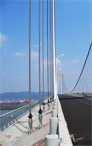
For the cables with fixed-fixed or hinged-fixed boundary conditions which are commonly used in real bridge structures (as Figs. 1 and 2 show), there are no analytical formulas to calculate their cable tensions from the measured frequencies. The third category formulas have been established to solve such problems. This is the so-called practical formulas.
Fig. 1The vertical cable used in arch bridge with fixed-fixed boundary conditions
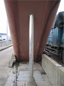
Fig. 2The vertical cable used in suspension bridge with hinged-fixed boundary conditions
Zui et al. [6] presented practical formulas to estimate the cable forces from the first and second natural frequencies of cable vibration as Eq. (3)-(5) show. The formulas are based on the approximate solutions of high accuracy for the equation of inclined cable with flexural rigidity. But for the vertical cables without sag-extensibility, these formulas can only use the fundamental frequency for calculation.
1. In the case of using the natural frequency of first-order mode (cable with sufficiently small sag ):
2. In the case of using the natural frequency of second-order mode (cable with relatively large sag ):
3. In the case of using the natural frequencies of high-order modes (very long cable ):
where , .
Mehrabi and Tabatabai [7] proposed a simple relationship among non-dimensional cable parameters for in-plane and out-of-plane vibration modes. The relationship accounts for both the sag-extensibility and bending stiffness effects. The cable ends are assumed to be fixed. This relationship is most accurate when (the sag-extensibility parameter) is less than 3.1 and is more than 50. The function is shown in Eq. (6):
In which:
Ren et al. [8] proposed empirical formulas to estimate cable tension based on the solutions by means of energy method and fitting the exact solutions of cable vibration equations, shown in Eqs. (7). The cable bending stiffness effect is taken into account. The empirical formulas to estimate cable tension are based on the cable fundamental frequency only:
Gan et al. [9] proposed a practical formula of cable tension estimation based on the vibration function of Euler-Bernoulli beam with fixed-fixed boundary conditions and energy principle. The expression is as Eq. (8) shows, it is very simple, but the precision is not very good [10]:
where , .
Fang et al. [11] proposed a practical formula with simple explicit form on the basis of the transverse vibration equation of a cable and by using a curve-fitting technique to replace the numerical iterative process. The formula is shown in Eq. (9). But the cable ends are assumed to be fixed, and therefore it can’t be used in other boundary conditions:
In which:
The aforementioned practical formulas all assumed the ends of cable are both fixed, so it can’t be used to estimate the tension of cables with hinged-fixed boundary conditions. Furthermore, most of the existing practical formulas can only use the fundamental frequency for calculation. But for in-situ test, sometimes the fundamental frequency is difficult to be measured for the reasons of excitation methods, sensor’s sensitivity, mounting position of the sensors and so on. If the fundamental frequency of cable is not obtained, the common method is using the frequency differences between two frequencies as the fundamental frequency. It may lead to unacceptable errors for the cables with large bending stiffness. So, new practical formulas which can solve those problems are needed.
The objective of this paper is to propose a new practical formula that can estimate cable tension from measured natural frequencies satisfying hinged-fixed boundary conditions. To achieve this objective, the following three tasks are performed. Firstly, from the general solution of the vibration equation of the vertical cable, practical formula of the cable tension identification satisfying hinged-fixed boundary conditions is derived. The expression of the practical formulas is the same as the solution derived from an axially loaded beam with simply supported ends and in which only an additional parameter is introduced. Secondly, by using Newton iterative method, the numerical solutions of the frequency equation of the tensioned vertical cable with hinged-fixed boundary conditions are obtained. By the least squares fitting method, and based on the theoretical results the relationship between and the cable’s geometrical and physical parameters is fitted. Thirdly, the feasibility and practicability of the proposed approach are examined through error analysis and by several numerical examples.
2. Basic governing equations and solutions
Vertical cables are mostly used in tied-arch bridges and suspension bridges, it have no sag, so the equation of lateral motion coincides with the equation of the motion of a beam with axial tension as follows [12]:
where is the bending stiffness of the cable, is the lateral deflection due to vibration, is the axial cable force, is the mass of cable per unit length.
Using the method of separation of variables, the general solution of Eq. (10) can be obtained as follows:
where:
Defined:
Eq. (11) can be rewritten as:
For hinged-fixed boundary conditions, the boundary conditions used to determine the constants through from Eq. (14) are:
The natural frequencies are obtained from the condition that the determinant of the boundary conditions is set equal to zero:
Frequency equations can be obtained from Eq. (16), as Eq. (17) shows:
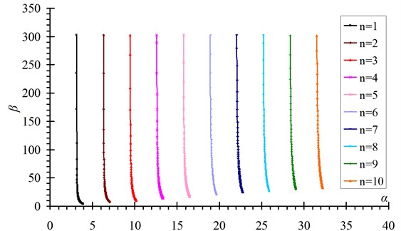
It is a transcendental equation, so no explicit solutions can be obtained. Newton iterative method is used to calculate the value of versus , the results of and for the first ten order modes are shown in Fig. 3.
Fig. 3The solutions of βn versus αn for hinged-fixed boundary conditions (n= 1-10)
3. Establishment of practical formulas
From Eqs. (12) and (13) we arrive at:
Combining Eqs. (18a) and (18b), can be solved as:
Defined , then:
Eq. (20) is the proposed practical formula to calculate cable tension. Compared with the pre-existing formulas, this formula is derived from the general solution of the equation of motion for a cable with axial tension , so it can be used for any constraint conditions in theory.
In Eq. (20), is an unknown parameter, for different conditions the value of is different. If the boundary is simple supported, then 1 and Eq. (20) becomes the same as Eq. (2). But for the hinged-fixed boundary conditions, is not a constant and can’t be solved directly. From the practical point of view, fitting formula to calculate the value of is needed based on the theoretical results.
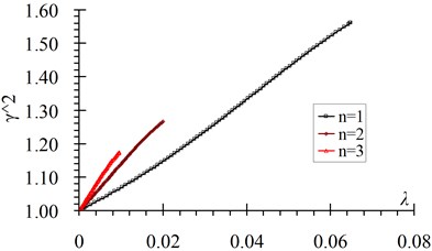
Fig. 4 shows the relationship between and for the first ten order modes of cables with hinged-fixed boundary conditions from the theoretical results. A quadratic best fit function is obtained between and in the form of Eq. (21):
where:
Fig. 4γn2-λn relation curves a) n= 1-3, b) n= 4-10
a)
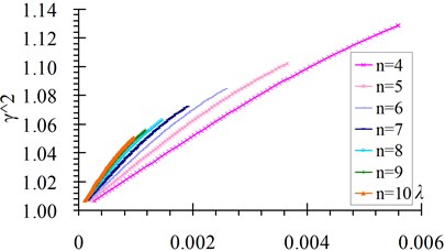
b)
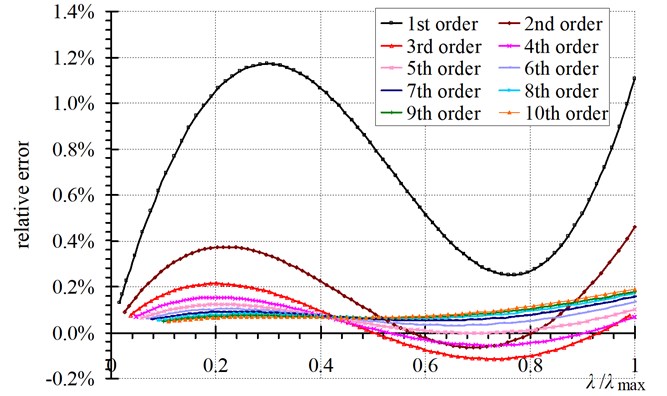
Fig. 5 shows the comparison curves between the theoretical value and fitted value. Fig. 6 shows fitting errors of versus . From these figures it can be seen that: 1) Fitted values coincide well with the theoretical values, the first order frequency has the maximum fitting error and the value is no more than 1.5 %; 2) Fitting errors decrease with the increase of the frequency order; 3) The errors of the 2-10 order frequencies are all less than 0.5 % in the whole range.
Fig. 5Comparisons of fitted value with theoretical value of γn2 versus λn: a) n= 1, b) n= 3, c) n= 5, d) n= 10
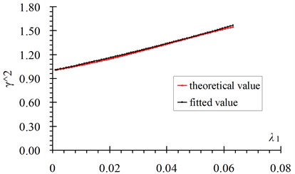
a)
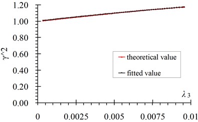
b)
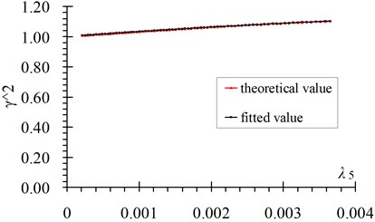
c)
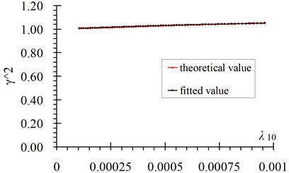
d)
Summarize the results aforementioned, the expression of practical formulas to calculate the tension of vertical cables for hinged-fixed boundary conditions is as follows:
In which:
Fig. 6Curves of relative errors of γn2 versus λ/λmax
The expression of Eq. (22) is the same as Eq. (2) which is derived from the vibration equation of axially loaded beam, with the difference that an additional parameter is needed. For hinged-hinged boundary conditions, 1. So Eq. (2) can be regarded as a special case of Eq. (3).
4. Error analysis
From the derivation process of the practical formula, it can be seen that if the frequencies are measured exactly and the structural parameters of the cable are accurate, the error of estimated cable tension is only resulted from the error of fitted and can be calculated theoretically.
From Eq. (23b) we obtained:
Submitting Eq. (24) into Eq. (22), then we arrive at:
Defining the relative error of is , so the calculated cable tension is:
Defined the error of is , then:
From Fig. 6, we can get the value of for a specified . Then the error of can be calculated by using the Eq. (27) and the known parameters. The curves of relative errors of versus are shown in Fig. 7.
Fig. 7Curves of relative errors of T versus λ/λmax
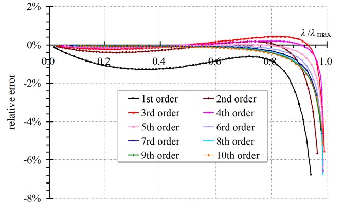
From Fig. 7 we can seen that: 1) The error of calculated with the fundamental frequency is larger than that calculated with other order frequencies. When , the errors of calculated with the fundamental frequency are less than 2 %; When , the errors are less than 5 %. 2) The errors of calculated with the 2-10 order frequencies have high precision. When , the errors of calculated with 2-10 order frequencies are all less than 1 %; When , the errors of calculated with 2-10 order frequencies are less than 5 %; When , the errors of calculated with 2-10 order frequencies become larger than 5 %, and increase rapidly.
From the definition of and , we arrive at:
is a non-dimensional parameter reflecting the effect of cable’s bending stiffness defined by Zui et al. [6]. In the common references, according to the value of , cables can be classified into several categories as shown subsequently. When is very large, the cable is called long cable and can be known as a taut string. When is very small, the cable is called short cable and can be known as an axially-tensioned beam. And when is between the two category defined above, the cable is called medium length cable and the dynamic behaviors of them are combined the property of axially-tensioned beam and taut string. In order to facilitate comparison with the references, the curves of relative errors of versus are obtained as shown in Fig. 8.
From Fig. 8 it can be seen that: 1) The errors of calculated cable tension decrease with the increase of ; 2) For the same value of , the errors of are different when using different order frequencies, in general, the order of frequency is higher, the error of is larger. When , the errors of the calculated cable tension using the first ten order of frequencies are all less than 5 %.
Table 1 lists the value of when the value of errors is 2 % and 5 %. From the table, if the value of is known, the error range of the calculated cable tensions can be pre-estimated. This is very useful in engineering applications. In practice, 5 % are usually used as the upper limit of allowable error. So from Table 1, we can see that the practical formulas in this paper is applicable when if the fundamental frequency is used to determine the cable force, and when , the errors of the calculated cable tension using the fundamental frequency are less than 2 %. Nearly all of the vertical cables used in bridge engineering are in this range. So the formulas in this paper have high precision in engineering application.
Fig. 8Curves of relative errors of T versus ξ
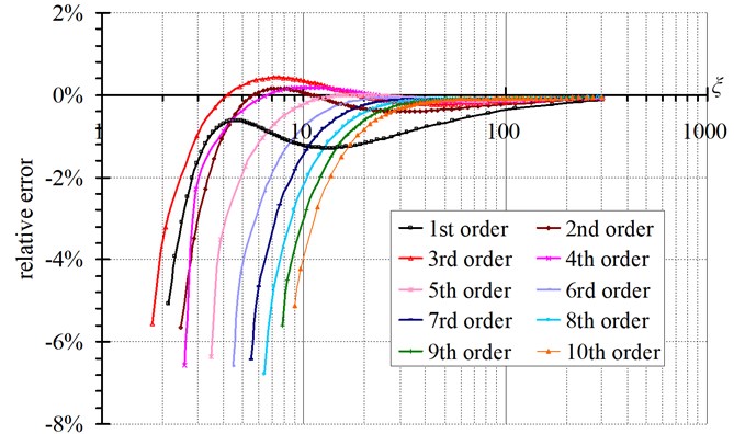
Table 1The value of ξ for specific value of errors
Error | ||||||||||
Frequency order | ||||||||||
1 | 2 | 3 | 4 | 5 | 6 | 7 | 8 | 9 | 10 | |
2 % | 2.8 | 3.3 | 2.5 | 3 | 4.9 | 6.7 | 8.6 | 10.5 | 12 | 13.5 |
5 % | 2.1 | 2.6 | 1.9 | 2.6 | 3.6 | 4.8 | 5.9 | 7.0 | 8.0 | 9.0 |
5. Identification of bending stiffness
The geometrical parameters of cables are very important in estimating cable tensions. Those parameters include the mass of the cable per unit length, the length of the cable, the bending stiffness of the cable and so on. Among these parameters, the bending stiffness is the most difficult to be obtained because most of cables are using parallel steel wire or steel stranded wire and the cross section of it no longer conform with the assumption of plane cross section. Bending stiffness has significant influence on cable force estimation especially for the short vertical cables, so identification of bending stiffness is very important to improve the accuracy of cable tension estimation. It can be identified by using the formulas in this paper with multiple natural frequencies. The principle of the identification is as follows:
From , we obtained:
Then can be solved:
Because , is a function of , Eq. (30) can’t be solved explicitly, iterative method is needed. The iterative steps are as follows:
1. The iterations start with initial value of , then substitute into Eqs. (23a) and (23b), , are calculated;
2. Substitute , in to Eq. (30), is obtained, if , then the bending stiffness is and the iteration is stopped. is a desired tolerance. Otherwise, completing the cycle of iteration to be repeated until the desired accuracy is attained.
6. Verification examples
From the product manual of hanging-cable/tied-cable system for arch bridge pressed by OVM company which is a professional manufacturer of steel strand in China [13], several hanging-cable styles commonly used in arch bridge are used as the verification examples. The hanging-cables are composed of 37-211 parallel wires and the length of the cable are in the range of 3 m to 70 m, which contained nearly all of the vertical cables used in tied-arch bridges.
6.1. Estimation of cable force
Table 2 shows the comparison results of the calculated cable tension using the formulas in this paper. From this table, it can be seen that the differences between the results of Eq. (2) and the exact value are very large and the differences are decreased with the value of increasing. For the cables with , the errors will be less than 5 %. So the precisions of calculated cable tensions using the presented formulas are improved largely. For all kinds of cables, the errors of the calculated results with all order frequencies are no more than 1.5 %. Especially for the cables with , the errors of the calculated cable tensions are less than 0.1 %.
Table 2Comparison of computed cable tensions
Cable type | (m) | (kg/m) | () | (kN) | (Hz) | Freq. order | Eq. (2) (kN) | Present method (kN) | Error of | Error of | |
PES(FD)7-37 | 3 | 13.6 | 34928 | 500 | 11 | 36.365 | 1 | 609 | 494 | 21.8 % | 1.3 % |
PES(FD)7-55 | 5 | 20.1 | 77195 | 1000 | 18 | 50.043 | 2 | 1137 | 997 | 13.7 % | 0.3 % |
PES(FD)7-73 | 10 | 26.6 | 135910 | 1500 | 33 | 38.185 | 3 | 1603 | 1497 | 6.9 % | 0.2 % |
PES(FD)7-91 | 15 | 33.5 | 211242 | 2000 | 46 | 34.522 | 4 | 2097 | 1997 | 4.9 % | 0.1 % |
PES(FD)7-109 | 20 | 39.3 | 303118 | 2500 | 57 | 33.274 | 5 | 2598 | 2498 | 3.9 % | 0.1 % |
PES(FD)7-127 | 30 | 46.4 | 411538 | 3000 | 81 | 26.444 | 6 | 3082 | 2999 | 2.7 % | 0.0 % |
PES(FD)7-151 | 40 | 54.1 | 581634 | 3500 | 98 | 23.055 | 7 | 3580 | 3500 | 2.3 % | 0.0 % |
PES(FD)7-187 | 50 | 66.9 | 892176 | 4000 | 106 | 20.31 | 8 | 4086 | 4001 | 2.2 % | 0.0 % |
PES(FD)7-199 | 60 | 71.0 | 1010133 | 4500 | 127 | 19.516 | 9 | 4583 | 4503 | 1.8 % | 0.1 % |
PES(FD)7-211 | 70 | 75.5 | 1135690 | 5000 | 154 | 19.825 | 10 | 5082 | 5006 | 1.6 % | 0.1 % |
6.2. Estimation of bending stiffness
If more than one order of frequencies were obtained, bending stiffness of cables can be identified by using the method presented in this paper. To verify the accuracy of bending stiffness identification method, cable 1 and cable 10 are analyzed as examples. Table 3 shows the comparison of identified value of . Table 4 gives the solution history of iteration when using the 1st and 2nd order of frequencies for cable 1.
From Table 3 it can be seen that: 1) Bending stiffness of cable 1 and cable 10 are accurately identified with the errors being no more than 10 %. 2) The error of the cable with larger is larger than that of the cable with smaller . This is because the bending stiffness has little impact on the estimation results for the cable with larger . In other words, the cable tension identification is insensitive to the change of cable’s bending stiffness for the cable with larger . Even the bending stiffness changed largely, the cable tension will change little. 3) The error of identified bending stiffness using the first order frequency is the largest. It is mainly because the fitted value of for the first order frequency is more roughly than the others which can be seen from Fig. 5.
From Table 4 we can see that the iteration of the method presented in this paper are converged quickly, and the satisfied results are obtained after only 5 steps of iterations.
Table 3Comparison of identified EI value
Cable 1 (PES(FD)7-37) | Cable 10 (PES(FD)7-211) | ||||||||
Freq. order | (Hz) | Ture value () | Identified value () | Relative error | Freq. order | (Hz) | Ture value () | Identified value () | Relative error |
1 | 40.168 | 34928 | 36535 | 4.6 % | 1 | 1.9571 | 1135690 | 1220137 | 7.4 % |
2 | 87.863 | 34928 | 2 | 3.9167 | 1135690 | ||||
3 | 148.02 | 34928 | 34866 | 0.2 % | 3 | 5.8812 | 1135690 | 1200290 | 5.7 % |
4 | 223.14 | 34928 | 4 | 7.8529 | 1135690 | ||||
5 | 314.45 | 34928 | 34776 | 0.4 % | 5 | 9.8344 | 1135690 | 1171519 | 3.2 % |
6 | 422.59 | 34928 | 6 | 11.828 | 1135690 | ||||
7 | 547.9 | 34928 | 34823 | 0.3 % | 7 | 13.836 | 1135690 | 1137662 | 0.2 % |
8 | 690.6 | 34928 | 8 | 15.861 | 1135690 | ||||
9 | 850.85 | 34928 | 34925 | 0.0 % | 9 | 17.906 | 1135690 | 1148930 | 1.2 % |
10 | 1028.8 | 34928 | 10 | 19.972 | 1135690 | ||||
Table 4Solution history of EI iteration
Iteration | Difference (%) | ||||||
1 | 0 | 0.000 | 0.000 | 1.00 | 1.00 | 41168 | 17.9 % |
2 | 41168 | 0.027 | 0.012 | 1.22 | 1.17 | 36409 | 4.2 % |
3 | 36409 | 0.025 | 0.011 | 1.20 | 1.16 | 36539 | 4.6 % |
4 | 36539 | 0.025 | 0.011 | 1.20 | 1.16 | 36535 | 4.6 % |
5 | 36535 | 0.025 | 0.011 | 1.20 | 1.16 | 36535 | 4.6 % |
7. Conclusions
Practical formula for cable tension identification satisfying hinged-fixed boundary conditions is proposed based on the general solution of the transverse vibration equation of the vertical cable. It is a unified formula with the same expression as the solution derived from an axially loaded beam with simply supported, without segmentation, and can be used to calculate tensions conveniently and accurately. Moreover it can be used to estimate the cable tension by directly using its first ten order frequencies and taking the bending stiffness into account. The capability of this formula has been verified through several numerical examples, which indicated that those formulas are sufficiently accurate and can be conveniently applied to in-situ measurement of vertical cables used in bridge structures.
The formula presented in this paper, originating from the theoretical solution with few approximations and assumptions, has high precision and the errors are only resulting from the error of coefficient fitting, and the error between the estimated results and the exact solutions can be calculated theoretically. For hinged-fixed conditions, when the cable’s dimensionless parameter , the errors of calculated cable tension using the first ten order of frequencies are all less than 5 %. If using the cable’s fundamental frequency to calculate, when the cable’s dimensionless parameter , the errors of calculated cable tension will be no more than 2 %. In a real bridge, most of their cables are tensioned to a relatively large internal force with its parameter in order to make the best use of the material. So, the practical formulas in this paper can be applied to estimate nearly all of the cable tension in real bridges conveniently and accurately.
The formula in this paper can be simultaneously used to identify the cable’s bending stiffness and force with multiple natural frequencies being measured. The iterative equation is derived and the iterative steps are given. From the example analysis it can be seen that the bending stiffness identification method presented in this paper is converged quickly, and the satisfied results can be obtained after only a few steps of iteration.
References
-
Sun Y., Li H. Effect of extreme properties of vertical cable on the cable force measurement by frequency-based method. Engineering Mechanics, Vol. 30, Issue 8, 2013, p. 10-17, (in Chinese).
-
Fei Q. G., Han X. L. Identification of modal parameters from structural ambient responses using wavelet analysis. Journal of Vibroengineering, Vol. 14, Issue 3, 2012, p. 1176-1186.
-
Kim B. H., Park T. Estimation of cable tension force using the frequency-based system identification method. Journal of Sound and Vibration, Vol. 304, Issue 3-5, 2007, p. 1067-1072.
-
Caetano E. On the identification of cable force from vibration measurements. IABSE-IASS Symposium, London, 2011.
-
Humar J.L. Dynamics of structures. Prentice Hall, Upper Saddle River, NJ, 1990.
-
Zui H., Shinke T., Namita Y. Practical formulas for estimation of cable tension by vibration method. Journal of Structural Engineering-ASCE, Vol. 122, Issue 6, 1996, p. 651-656.
-
Mehrabi A. B., Tabatabai H. Unified finite difference formulation for free vibration of cables. Journal of Structural Engineering-ASCE, Vol. 124, Issue 11, 1998, p. 1313-1322.
-
Ren W. X., Chen G., Hu W. H. Empirical formulas to estimate cable tension by cable fundamental frequency. Structural Engineering and Mechanics, Vol. 20, Issue 3, 2005, p. 363-380.
-
Gan Q., Wang R. H., Rao R. Practical formula for estimation on the tensional force of cable by its measured natural frequencies. Chinese Journal of Theoretical and Applied Mechanics, Vol. 42, Issue 5, 2010, p. 983-988, (in Chinese).
-
Tang S. H., Fang Z., Yang S. Practical formula for the estimation of cable tension in frequrency method considering the effects of boundary conditions. Journal of Hunan University, Natural Sciences, Vol. 39, Issue 8, 2012, p. 7-13, (in Chinese).
-
Fang Z., Wang J. Q. Practical formula for cable tension estimation by vibration method. Journal of Bridge Engineering-ASCE, Vol. 17, Issue 1, 2012, p. 161-164.
-
Clough R. W., Penzien J. Dynamics of structures. McGraw-Hill, New York, 1993.
-
OVM Engineering Co., LTD. Product manuals of hanging-cable/tied-cable system for arch bridge. Liuzhou OVM Engineering Co., LTD, LiuZhou, China, 2007, (in Chinese).
About this article

The authors gratefully acknowledge the financial support by Project supported by the National Natural Science Foundation of China (Grant No. 51208123; No. 51208229), the Project supported by the Natural Science Foundation of Guangdong Province, China (Grant No. S2012040007317), and the Talent Introduction Project supported by Higher Education Department of Guangdong Province in 2012.
