Abstract
Numerical cases of the use of natural frequencies to identify crack location and crack depth in beams under noise-free conditions have been widely reported. However, the capability of natural frequencies to identify cracks in noisy conditions has not yet been systematically addressed. Unlike previous work stressing the merits of natural frequencies in depicting cracks, this study reports the performance assessment of natural frequencies in characterizing cracks in noisy conditions. In the performance assessment, a cracked cantilever Timoshenko beam, with the crack flexibility modeled by fracture mechanics principles, is considered. The results demonstrate quantitatively and exhaustively that natural frequencies, as global dynamic properties of a structure, are somewhat insensitive to local slight damage. The outcome of this study provides a guideline for rational use of natural frequencies to identify cracks in actual beam-type structures.
1. Introduction
Structural damage detection has been a research focus of increasing interest in mechanical, civil, aerospace, and military fields during the last few decades [1-8]. A crack in a structural member increases its local flexibility [9], which necessarily causes changes in structural dynamic properties such as modal parameters [10, 11], from which the location and extent of the crack can be identified [12]. Among various modal parameters, natural frequency is the feature most frequently used to identify cracks, due to its reliability and facilitation in acquisition [13]. In the last two decades, the identification of cracks in beams based on natural frequencies has been increasingly investigated in the structural health monitoring community [14, 15]. The most representative method of using natural frequencies to identify cracks in a beam is the frequency contour method [16-24]. This method estimates the location and extent of a crack in a beam using measurements of natural frequencies, incorporating an analytical model of the beam. The frequency contours of crack depth versus crack location are commonly plotted for the first three natural frequencies and the intersection points of the contours graphically indicate the location and depth of the crack being inspected.
The development of the frequency contour method can be summarized as follows. Liang et al. [16] originated the method using an analytical model of an Euler-Bernoulli beam, and demonstrated the validity of the method through cracked beam cases. Nandwana and Maiti [17] accentuated the positive effect of ‘zero setting’ for enhancing the accuracy of the method in identifying cracks in stepped beams [18]. Lin [19] advanced the method replacing Euler-Bernoulli beam theory with Timoshenko beam theory, which is applicable to short-thick beams and high-frequency vibration of long-thin beams that behave like a set of short-thick beams. As well, Chinchalkar [20] gave the method greater generality by adopting a finite element model rather than analytical beam theories for beam modeling. Parallel to the development of the method itself, applications of the frequency contour method have been much reported in the literature [21-24], commonly concentrating on providing a group of analytical or numerical cases of successful identification of crack in beams.
Despite their popularity for characterizing damage, performance assessment of natural frequencies in identifying cracks is still pending. In essence, several factors influence the capacity of natural frequencies to depict damage: (i) as reported in [11], natural frequencies are somewhat insensitive to slight damage [12]; (ii) experimentally measured natural frequencies cannot accurately reflect the inherent frequencies of structures due to the interference of measurement error and uncertainty; (iii) the simplifications of beam theories make crack modeling more or less inaccurate. These factors may impair the effectiveness of natural frequencies in identifying cracks in beams. It is of great significance, therefore, to assess the performance of natural frequencies in characterizing damage, so as to provide a guideline for reasonable use of this feature in practical damage diagnosis.
2. Formulation
As per Timoshenko beam theory, the equations of motion for a Timoshenko beam are given as:
where is the transverse displacement of an arbitrary point of the beam at the moment , the angle of rotation caused by bending, the modulus of elasticity, the shear modulus, the area moment of inertia, the mass density of the material, the cross-sectional area, and the shear coefficient.
The dimensionless height and length of a beam are represented as and , with and being the beam height and beam length, respectively. By introducing the following variables, with being the natural angular frequency:
and the general solution of Eqs. (1a) and (1b) is given as [25, 26]:
where and are the amplitude functions of and , respectively. , , are arbitrary constants to be determined by boundary conditions.
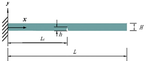
With Timoshenko beam theory, the equations of motion for a Timoshenko beam containing a crack can be formulated as follows. A uniform rectangular-sectional cantilever beam with a through-width single-sided crack (Fig. 1) is considered, where and denote the location and depth of the crack, respectively. The crack can be further depicted by two dimensionless parameters, crack location ratio, i.e., , and crack depth ratio, i.e., . In terms of Eqs. (3a) and (3b), the equations of motion for the two beam segments joined by the crack can be expressed as [19, 27, 28]:
where and , , are arbitrary constants to be determined by the continuity conditions at the crack and the boundary conditions of the beam.
Fig. 1A two-segment beam model with a massless rotational spring
a)
b)
The conditions of continuity of displacement, moment, and shear force at the crack are given as:
The discontinuity in the slope at the crack is specified by:
where is the dimensionless crack-sectional flexibility in the form [29]:
with expressed as:
The boundary conditions for the cantilever beam are given as:
Using the transfer matrix method [19] together with the continuity and boundary conditions, i.e., Eqs. (5)-(9), the characteristic equation can be represented in the form [27]:
with and detailed as:
The characteristic equation described in Eq. (10) is essentially an analytical function with respect to natural frequency (), crack location ratio () and crack depth ratio (). For clarity, Eq. (10) can be further represented as:
Equation (12) potentially provides a mechanism for identifying a crack in a beam using measured natural frequencies. With several natural frequencies inputted into Eq. (12), a system of simultaneous characteristic equations (Eq. (12)) can be created. Theoretically, solving this system can determine the unknown crack parameters, and . In what follows, this mechanism of crack identification is clarified in detail.
3. Advanced frequency contour method
3.1. Frequency contour method
3.1.1. Exact natural frequencies
Generally, the frequency contour method needs three natural frequencies to form an over determined system of simultaneous characteristic equations with two unknowns of crack parameters, and The solution of the system specifies the estimated crack parameter. Assuming , and are the first three measured natural frequencies that exactly reflect the real frequency characteristics of the beam being diagnosed, these frequencies can frame a system:
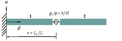
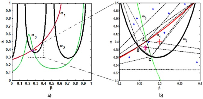
For a natural frequency , the possible solutions of unknown crack parameters arising from constitute a set that forms a frequency contour in the domain, as that labeled by , or in Fig. 2(a). Physically, there is only one group of and that simultaneously satisfies the system defined by Eq. (13), such that the intersection point of these frequency contours can identify the crack, as illustrated in Fig. 2(a).
Fig. 2Crack identification from frequency contours with exact (a) and noisy (b) natural frequencies (+: actual crack; *: identified crack)
(a)
(b)
3.1.2. Noisy natural frequencies
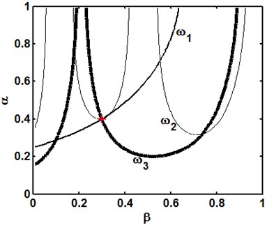
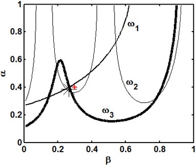
In practical damage diagnosis, noise is unavoidably present in measured natural frequencies, leading to noisy natural frequencies, , , , deviated from the exact natural frequencies. Using , , instead of , , to set up the characteristic equations in Eq. (13), gives:
where and denote the crack parameters determined by the noisy natural frequency. Owing to the noise effect, the three frequency contours resulting from Eq. (14) do not exactly intersect at a sole point (Fig. 2(b)), but they produce a series of intersectional triangles. As suggested by Nandwana and Maiti [17], the centroid of a certain correct intersectional triangle can be used to estimate the crack parameters (Fig. 2(b)). The issue of judiciously determining the correct intersectional triangle from all possible cases is, however, not yet resolved [18].
3.2. Advanced frequency contour method
Because of the noise present in measured , , , the frequency contours of , , and have multiple intersection points, as illustrated in Fig. 3(a) where eight intersection points can be found. Any three of these points can form an intersectional triangle, and therefore a series of intersectional triangles can be obtained from all the intersection points. For these triangles, it is difficult to visually select the correct one whose centroid can be used to estimate the crack parameters. To this end, a smallest-area principle is created for to facilitate the selection of the correct triangle. The area of an intersectional triangle quantifies the concentration of the three intersection points. A smaller area indicates greater closeness of the three points, and in turn may produce a more accurate estimation of crack parameters from the centroid. That being the case, a smallest-area principle can be set up to distinguish the correct intersectional triangle from all candidates. By way of illustration, the possible intersection triangles within the area of the dot-line-side rectangular in Fig. 3(a) are detailed in Fig. 3(b), where the dash-dot line labels the side of intersectional triangles, the asterisk denotes the centroid of an intersectional triangle, the plus sign specifies the actual crack parameters, and the triangle ABC represents the identified correct intersectional triangle, of which the centroid gives the estimate of crack parameters.
Aided by this smallest-area principle, a advanced frequency contour method is created and implemented using Matlab® language to automatically estimate the crack parameters for a beam. This advanced frequency contour method includes two distinctive features: (i) the vectorization capabilities of Matlab® place a high priority on efficiency in calculating the intersection points so as to form all the intersectional triangles, with the centroid marked by an asterisk for each triangle (Fig. 3); and (ii) the smallest-area principle is precisely activated to determine the crack parameters.
Fig. 3Crack identification using advanced frequency contour method. (a) F1(ω1*,e*,η*), F2(ω2*,e*,η*), and F3(ω3*,e*,η*) intersect at multiple points; (b) asterisk-labeled intersectional triangles within the area of the dot-line-side rectangular in (a) and the correct intersectional triangle ABC for damage identification (-.-: side of intersectional triangle, *: centroid of triangle, +: actual crack, ABC: correct intersectional triangle)
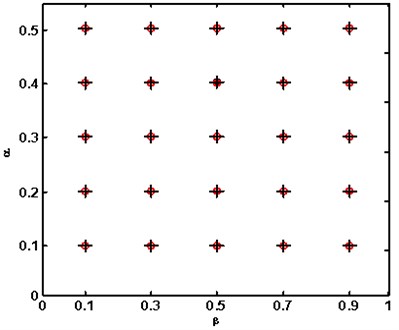
The accuracy of the advanced frequency contour method in crack identification in a cantilever beam with the basic parameters reported in [12] is demonstrated in Fig. 4, where each identified result labeled by a circle coincides well with the actual crack marked by a cross.
Fig. 4Demonstration of accuracy of advanced frequency contour method (o: actual cracks; +: identified cracks)
4. Performance assessment
The performance of natural frequencies in characterizing cracks is assessed using the advanced frequency contour method. The cantilever beam specimen described by Rizo et al. in [12] is considered, for which the elastic and geometric properties are: cross-section 20×20 mm2, length 300 mm, modulus of elasticity N/m2, density Kg/m3, Poisson ratio , shear modulus N/m2, and shear coefficient . Various crack cases are elaborated in light of crack location ratios of 0.2, 0.4, and 0.6, each with crack depth ratios 0.1, 0.2, 0.3, 0.4 and 0.5. The effect of a crack on the dynamic property is first evaluated by an index of frequency change ratio, , defined as:
where and are the th order natural frequencies for the intact and cracked beams, respectively. The resulting analytical natural frequencies and frequency change ratios for various crack cases are listed in Table 1.
Table 1Analytical natural frequencies and frequency change ratios for various cracks
Case No. | Analytical natural frequencies (Hz) | Frequency change ratios (%) | |||||
Position () | Depth () | ||||||
0.2 | 0.1 | 182.77 | 1140.92 | 3116.17 | 0.67 | 0.02 | 0.22 |
0.2 | 179.33 | 1140.21 | 3097.33 | 2.54 | 0.09 | 0.82 | |
0.3 | 173.61 | 1139.05 | 3066.37 | 5.65 | 0.19 | 1.81 | |
0.4 | 165.37 | 1137.44 | 3022.70 | 10.1 | 0.33 | 3.21 | |
0.5 | 154.76 | 1135.47 | 2968.85 | 15.9 | 0.50 | 4.94 | |
0.4 | 0.1 | 183.51 | 1136.01 | 3114.23 | 0.27 | 0.46 | 0.28 |
0.2 | 182.07 | 1121.82 | 3090.49 | 1.05 | 1.70 | 1.04 | |
0.3 | 179.58 | 1098.45 | 3052.79 | 2.41 | 3.75 | 2.25 | |
0.4 | 175.72 | 1065.26 | 3002.21 | 4.51 | 6.65 | 3.87 | |
0.5 | 170.25 | 1023.71 | 2943.64 | 7.48 | 10.3 | 5.74 | |
0.6 | 0.1 | 183.89 | 1134.38 | 3111.07 | 0.07 | 0.60 | 0.38 |
0.2 | 183.52 | 1115.53 | 3078.92 | 0.27 | 2.25 | 1.41 | |
0.3 | 182.88 | 1083.95 | 3028.29 | 0.61 | 5.02 | 3.03 | |
0.4 | 181.84 | 1037.94 | 2961.25 | 1.18 | 9.05 | 5.18 | |
0.5 | 180.27 | 978.33 | 2885.01 | 2.03 | 14.30 | 7.62 | |
Intact | – | 184.01 | 1141.2 | 3123.0 | – | – | – |
4.1. -noise cube
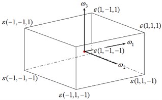
For performance assessment, identifications of cracks at various noise levels are implemented. A -noise cube is proposed to depict the noise effect involved in actual experimental measurements. The -noise cube is defined by:
where , , is the exact first three natural frequencies of the cracked Timoshenko beam model, and , , are the possible values arising from actual measurement. According to the -noise cube, there are eight possible deviations of from , specified by the vertices of the cube. Consequently, eight groups of , , are required in light of the -noise cube to bound the possible variations of actual measurement for each crack case at a specified level of noise.
Fig. 5ε-noise cube
4.2. Crack identification
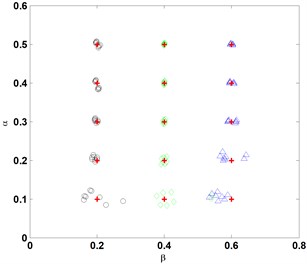
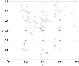
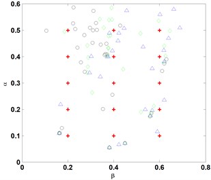
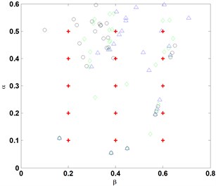
The procedure of identifying a crack using the advanced frequency contour method, as described in Section 3.2, is implemented independently for every crack case listed in Table 1. For each case, eight groups of , , are produced at a noise level in terms of the -noise cube, correspondingly giving rise to eight groups of estimates of crack parameters, and . These estimates jointly characterize the result of crack identification at a certain noise level. When noise level varies from 1/10000 to 6/100, the representative results of crack identification are shown in Fig. 6, from which several observations can be derived:
(1) Accuracy of crack identification gradually decreases with the increase in noise level;
(2) Accuracy of crack identification progressively increases with the increase in crack depth;
(3) When the noise level exceeds 3/1000, the frequency contour method is basically incapable of identifying a crack with a crack depth ratio less than 0.1; and
(4) When the noise level exceeds 3/100, the frequency contour method is unable to identify a crack with a crack depth ratio less than 0.3.
To assess the accuracy of crack identification quantitatively, the indices of averaged identification error of the crack location, , and averaged identification error of the crack depth, , are created from the eight groups of identified and :
where and are the actual and identified crack location ratios, respectively; and are the actual and identified crack depth ratios, respectively.
The thresholds, and , are employed to distinguish successful cases () from unsuccessful ones () for crack location identification and successful cases () from unsuccessful () ones for crack depth identification, respectively. These thresholds are set up based on that 10 percent of beam length is the critical size of acceptable precision of crack location identification, and 5 percent of beam height is the critical size of acceptable precision of crack depth identification.
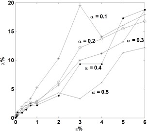
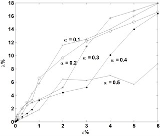
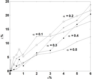
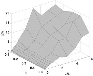
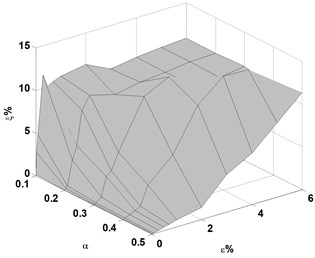
The indices, i.e., and , are evaluated for each case of crack identification. When noise level ranges from 1/10000 to 6/100, typical results of and are displayed in Figs. 7 and 8 for crack location ratios 0.2, 0.4, and 0.6, respectively. From these results, the following observations can be derived:
(1) For a crack case, the averaged identification error of the crack location or crack depth, or , increases with the increase in noise level;
(2) For cracks with identical location, the averaged identification error of crack location or crack depth, or , increases with the reduction in crack depth;
(3) For cracks with a crack depth ratio over 0.2, the noise tolerance for identifying location is greater than that for identifying depth. This means that crack depth is more difficult to identify than crack location; and
(4) For a cantilever beam, when cracks located further from the fixed end of the beam, the noise tolerances for identifying crack location and crack depth are both decreased.
Fig. 6Identification of cracks at various noise levels, where +: denotes the actual crack, and ○, ◊, and Δ: denote the identified cracks at e= 0.2, 0.4, and 0.6, respectively
(a)
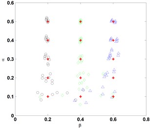
(b)
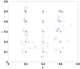
(c)
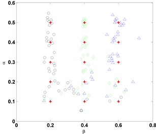
(d)
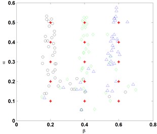
(e)
(f)
(g)
(h)
Fig. 7Variations of averaged identification error of crack depth, λ, with noise level, ε, for cracks of various depths located at e= 0.2, 0.4, and 0.6, respectively
(a)
(b)
(c)
Fig. 8Variations of averaged identification error of crack location, ξ, with crack depth, η, and noise level, ε, for cracks located at e= 0.2, 0.4, and 0.6, respectively
(a)
(b)
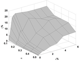
(c)
5. Conclusions
This study presents performance assessment of natural frequencies in characterizing damage of beams in noisy conditions. The performance assessment is implemented using an advanced frequency contour method, developed to estimate the location and depth of a crack in a beam in an entirely automatic manner. Sensitivity to damage and robustness against noise of natural frequencies are investigated through analyzing various crack scenarios incorporating the noise effect in measurements. The observations obtained provide a guideline for the reasonable use of natural frequencies to locate and quantify damage in beam-type structures.
References
-
Viet Ha N., Golinval J.-C. Damage localization in linear-form structures based on sensitivity investigation for principal component analysis. Journal of Sound and Vibration, Vol. 329, 2010, p. 4450-4566.
-
You Q., Shi Z. Y., Shen L. Damage detection in time-varying beam structures based on wavelet analysis. Journal of Vibroengineering, Vol. 14, 2012, p. 292-304.
-
Elenas A., Meskouris K. Correlation study between seismic acceleration parameters and damage indices of structures. Engineering Structures, Vol. 23, 2001, p. 698-704.
-
Alvanitopoulos P. F., Andreadis I., Elenas A. Neuro-fuzzy techniques for the classification of earthquake damages in buildings. Measurement, Vol. 43, 2010, p. 797-809.
-
Fayyadh M. M., Razak H. A. Damage identification and assessment in RC structures using vibration data: a review. Journal of Civil Engineering and Management, Vol. 19, 2013, p. 375-386.
-
Xiang J. W., Matsumotoa T., Wang Y. X., Jiang Z. S. Detect damages in conical shells using curvature mode shape and wavelet finite element method. International Journal of Mechanical Sciences, Vol. 66, 2013, p. 83-93.
-
Kim J. B., Eun H. C. Damage detection based on the internal force or deformation variation. Journal of Vibroengineering, Vol. 14, 2012, p. 350-314.
-
Wang S. S., Ren Q. W., Qiao P. Z. Structural damage detection using local damage factor. Journal of Vibration and Control, Vol. 12, 2006, p. 955-973.
-
Dimarogonas A. D. Vibration of cracked structures – a state of the art review. Engineering Fracture Mechanics, Vol. 5, 1996, p. 831-857.
-
An Y. H., Ou J. P. Experimental and numerical studies on model updating method of damage severity identification utilizing four cost functions. Structural Control and Health Monitoring, Vol. 20, 2013, p. 107-120.
-
Cao M. S., Ye L., Zhou L. M., Su Z. Q. Sensitivity of fundamental mode shape and static deflection for damage identification in cantilever beams. Mechanical Systems and Signal Processing, Vol. 25, 2011, p. 630-643.
-
Rizo P., Aspragathos N., Dimarogonas A. D. Identification of crack location and magnitude of a cantilever beam from vibration modes. Journal of Sound and Vibration, Vol. 138, 1990, p. 381-388.
-
Salawu O. S. Detection of structural damage through changes in frequency: a review. Engineering Structures, Vol. 19, 1997, p. 718-723.
-
Xu G. Y., Zhu W. D., Emory B. H. Experimental and numerical investigation of structural damage detection using changes in natural frequencies. ASME Journal of Vibration and Acoustics, Vol. 129, 2007, p. 686-700.
-
Kawamura S., Sakai K., Suzuki Y., Minamoto H. Proposition of a stepwise diagnosis method for a cracked beam using a force identification approach. Journal of System Design and Dynamics, Vol. 5, Issue 7, 2011, p. 1518-1530.
-
Liang R. Y., Choy F. K., Hu J. L. Detection of cracks in beam structures using measurements of natural frequencies. Journal of the Franklin Institute, Vol. 328, 1991, p. 505-518.
-
Nandwana B. P., Maiti S. K. Detection of the location and size of a crack in stepped cantilever beams based on measurements of natural frequencies. Journal of Sound and Vibration, Vol. 203, 1997, p. 435-446.
-
Adams R. D., Cawley P., Pye C. J., Stone B. J. A vibration technique for non-destructively assessing the integrity of structures. Journal of Mechanical Engineering Science, Vol. 20, 1978, p. 93-100.
-
Lin H. P. Direct and inverse methods on free vibration analysis of simply supported beams with a crack. Engineering Structures, Vol. 26, 2004, p. 427-436.
-
Chinchalkar S. Determination of crack location in beams using natural frequencies. Journal of Sound and Vibration, Vol. 247, 2001, p. 417-429.
-
Kim J.-T., Stubbs N. Crack detection in beam-type structures using frequency data. Journal of Sound and Vibration, Vol. 259, 2003, p. 145-160.
-
Morassi A., Rollo M. Identification of two cracks in a simple supported beam from minimal frequency measurements. Journal of Vibration and Control, Vol. 7, Issue 5, 2008, p. 729-739.
-
Patil D. P., Maiti S. K. Detection of multiple cracks using frequency measurements. Engineering Fracture Mechanics, Vol. 70, 2003, p. 1553-1572.
-
Patil D. P., Maiti S. K. Experimental verification of a method of detection of multiple cracks in beams based on frequency measurements. Journal of Sound and Vibration, Vol. 281, 2005, p. 439-451.
-
Huang T. The effect of rotary inertia and of shear deformation on the frequency and normal mode equations of uniform beams with simple end conditions. Journal of Applied Mechanics, Vol. 53, 1961, p. 579-584.
-
Han S. M., Benaroya H., Wei T. Dynamics of transversely vibrating beams using four engineering theories. Journal of Sound and Vibration, Vol. 225, Issue 5, 1999, p. 935-988.
-
Khaji N., Shafiei M., Jalalpour M. Closed-form solutions for crack detection problem of Timoshenko beams with various boundary conditions. International Journal of Mechanical Sciences, Vol. 51, 2009, p. 667-681.
-
Haisty B. S., Springer W. T. A general beam element for use in damage assessment of complex structures. Journal of Vibration, Acoustics, Stress and Reliability in Design, Vol. 110, 1988, p. 389-394.
-
Ostachowitz W. M., Krawczuk M. Analysis of the effect of cracks on the natural frequencies of a cantilever beam. Journal of Sound and Vibration, Vol. 150, 1991, p. 191-201.
About this article

This study was partially supported by the Key Program of National Natural Science Foundation of China (Grant No. 11132003), the partial support provided by a Foundation for the Author of National Excellent Doctoral Dissertation of P. R. China (Grant No. 201050), and a National Natural Science Foundation of China (Grant No. 11172091).
