Abstract
The governing equation of flow-induced vibration is deduced in terms of Hamilton’s principle for a variable diameter pipe conveying axial steady flow. Frobenius method is applied to analyze the governing equation. After the recursion formulas of coefficients are obtained, dynamic stiffness method is proposed for free vibration analysis of the variable diameter pipe conveying fluid. In the example, the natural frequencies of uniform pipes conveying fluid are computed and comparisons are made to validate the dynamic stiffness method. Then, the natural frequencies and modal shapes are obtained for the variable diameter pipe conveying fluid with different section variation coefficients and fluid velocities.
1. Introduction
Fluid-conveying pipe is widely used in nuclear industry, petroleum industry, and many other industries. The failure caused by the interaction between fluid and pipe wall occurs very frequently in practice. So flow-induced vibration of pipe conveying fluid attracts more and more interests of researchers. Ashley and Haviland [1] begun the research of bending vibrations of pipe line containing flowing fluid. Paidoussis [2] has studied the dynamic characteristics of pipe conveying fluid for many years, the great achievement he accomplished in nonlinear vibration of pipes set the foundation of pipe dynamics. Recently, flow-induced vibration of pipe conveying fluid is researched more exhaustively. Doare et al. [3] studied the dissipation effect on the local and global stability of pipe conveying fluid and proposed a numerical method to analyze the stability of finite-length system. Jung, Chung [4] investigated the stability of semi-circular pipe conveying harmonically oscillating fluid. They considered the extensibility and nonlinearity of the fluid-conveying pipe with different boundary conditions through Hamilton principle. Rinaldi, Prabhakar [5] studied micro-scale resonators containing internal flow, modeled as micro-fabricated pipe conveying fluid, and investigated the effects of flow velocity on damping, stability, and frequency shift. Huang, Liu [6] studied the natural frequencies of fluid conveying pipe with different boundary conditions through Garlerkin approach. Ragulskis, Fedaravicius [7] have developed a harmonic balance method in the FEM analysis of the fluid in pipe with taking the interactions between the vibrating pipe and fluid flow into consideration.
Uniform pipe was always adopted in the flow-induced vibration analysis of pipe conveying fluid. However, fluid-conveying pipes with variable section are widespread in nuclear engineering, such as pipe-expanding and nozzle etc. Hannoyer and Paidoussis [8, 9] have studied the dynamics of a slender tapered beam with internal and external flow in theory and experiment. Based on the researches of Hannoyer and Paidoussis [8, 9], we studied the dynamic characteristics of variable diameter pipes conveying fluid through stiffness matrix method. Natural frequencies and modal shapes of the variable diameter pipe were calculated in this paper and contrasts were made between the results in this paper and previous researches, which prove that the method employed in this paper is reasonable.
2. Motion equation of variable diameter pipe conveying fluid
Here, we use Hamilton’s principle to build the dynamic model of variable diameter pipe conveying fluid. Because that the fluid-conveying pipe is an open system. The Hamilton’s principle for open system is used here, i.e.:
where, is the system’s Lagrange function, that is , where , stand for the kinetic energy and potential energy of the system respectively. is the work done by non-conservative force, is the fluid mass per unit length, is the position vector of pipe exit. is the unit vector in tangent direction of the deformed pipeline, as shown in Fig. 1.
In the coordinate shown in Fig. 1, the absolute fluid velocity can be written as follow:
In Eq. (2), stands for the velocity of the fluid relative to the pipe. and are unit vectors in - and -directions. and stand for the partial derivatives with respect to (coordinate) and (time). According to the law of conservation of fluid mass, as shown in Eq. (3), the velocity of the fluid is change along the length of the conical pipe. So we use and here:
where is a constant.
Fig. 1The displacement sketch of simply supported pipe
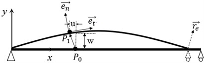
Fig. 2The sketch of variable diameter pipe
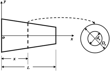
The sketch of a variable diameter pipe is shown in Fig. 2. The fluid flows from left end to right end. The outer and inner diameters of left end of the pipe are and respectively. The non-uniformity of the pipe is characterized by the diameter variation coefficient . The outer and inner diameters of the section at coordinate can be expressed as and respectively, where is length of the pipe. Because that the area of the fluid is , the velocity of the fluid along the length of the pipe can be expressed as:
Given that the flow velocity at the entrance of the pipe is , then Eq. (4) can be transformed into following form:
Now, we use Hamilton’s principle for open system to deduce the motion equation of variable diameter pipe conveying fluid. The kinetic energy of fluid in pipe can be written in the following form:
Here, the axial inextensible assumption was used, i.e. . And high order infinitesimals have been ignored in Eq. (6). is the density of fluid in pipe, is area of the fluid section located at . is mass of the fluid element analyzed.
The kinetic energy of the pipe is as follow:
where, is density of the pipe material, is area of the pipe cross section at . is mass of the pipe element.
The potential energy of the pipe is as follow:
In Eq. (8), is the inertial moment of the pipe section. Obviously, also changes along axis. Only considering the work done by fluid pressure, the work done by non-conservative force is zero [2], that is:
Substituting Eq. (6)-(9) into Eq. (1), the following equation can be obtained:
Here, we take the simply supported pipe (as shown in Fig. 1) for example to deduce the lateral vibration equation of the variable diameter pipe conveying fluid.
The boundary conditions of simply supported pipe are:
At time and
Combine Eq. (11) with Eq. (12), the following equation is obtained:
The detail manipulation of the third term in Eq. (10) is as follow:
Considering the assumption of axial inextensible, we obtain that , where the subscript ‘’ means “exit”, and the following equation can be gained:
Now, we can get the motion equation of variable diameter pipe conveying fluid as follow:
3. Free vibration analysis of variable diameter pipe
3.1. Frobenius method
To harmonic vibration, we have:
Substituting Eq. (17) into Eq. (16), we can get the following ordinary differential equation:
where:
and
For the purpose of analyzing Eq. (18) conveniently, the following dimensionless parameters are introduced here:
The dimensionless form of Eq. (18) is as follow:
Given that the contraction angle of the conical pipe is very small, that is, () is sufficiently small so that we can use Tylor series here as:
Here, we apply Frobenius method to analyze Eq. (22). Given that the solution of Eq. (22) takes the following form:
In which is the coefficient of the polynomial. The derivatives of are:
When , substituting Eq. (24) and Eq. (25) into Eq. (22), because that the lowest power of equals to zero, so the following equation can be obtained:
Because that , so we obtain:
Eq. (27) is namely indicial equation and it plays an important role in the analysis [10]. Obviously, Eq. (27) have four roots, i.e. 0, 1, 2, 3 (1, 2, 3, 4) respectively. To each , only one coefficient is related. Substituting Eq. (24) and Eq. (25) into Eq. (22), then all the coefficients can be obtained:
where:
Here, the high orders of have been neglected. After getting these coefficients, the solution of Eq. (22) can be written in the following form:
where is constant. The expression of is as follow:
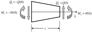
Fig. 3The sketch of node force
3.2. Dynamic stiffness method
Here, we use dynamic stiffness method to analyze vibration of variable diameter pipe conveying fluid. As shown in Fig. 3, the node displacement of the pipe is:
where:
As shown in Fig. 3, the shear force and bending moment can be expressed as:
Introducing the dimensionless form of shear force and bending moment as follows:
The directions of , are shown in Fig. 3, then it is easy to get the vector of node force:
where , , , .
The relation between vector of node force and vector can now be expressed as follow:
where:
In which , , and what should be noted here is that, stands for the derivative with respect to , which is different from that in Section 2.
According to Eq. (32), we can get the coefficient vector as follow:
Now, substituting Eq. (39) into Eq. (37), the following result will be gained:
Here, the matrix is named as the dynamic stiffness matrix of the system. Once the dynamic stiffness matrix is obtained, the natural frequencies and modal shapes can be easily obtained.
Here, we take the simply supported pipe for an example to illuminate how to compute natural frequencies of the pipe through dynamic stiffness method. The boundary conditions of simply supported pipe can be written as:
Rewriting Eq. (41) in the matrix form, we have:
The following characteristic equation can be obtained from Eq. (42):
It is easy to find from Eq. (43) that the following equation must be satisfied:
The natural frequencies can be obtained from Eq. (44). In the same way, we can get the characteristic equation for cantilevered pipe and clamped-pinned pipe conveying fluid as follows:
Cantilevered pipe (left clamped and right free):
Clamped-pinned pipe (left clamped and right pinned):
4. Examples
4.1. Uniform pipe conveying fluid
In order to validate the proposed method, we calculated the natural frequencies of a uniform pipe conveying fluid. The uniform pipe is actually the case of variable diameter pipe with section variation coefficient . The pipe and fluid parameters are chosen the same as previous reference, that is, Yang’s modulus is , the outer and inner diameters at origin of the pipe are and respectively, and the pipe span is , the density of pipe material is , the density of fluid is [11]. The first five orders of natural frequencies are computed under three different velocities, i.e. , , respectively. And comparisons are presented between the results obtained by the proposed method and that published in the research of Housner [11]. The computation results of natural frequencies and error are listed in Table 1.
Table 1Natural frequencies of uniform simply supported pipe conveying fluid under different fluid velocities (rad/s)
Fluid velocity | Natural frequency | |||||
This paper | 4.373 | 17.493 | 39.359 | 69.971 | 109.330 | |
Reference | 4.3732 | 17.4928 | 39.3587 | – | – | |
error (%) | 0.004 | 0.001 | 0.0007 | – | – | |
This paper | 4.287 | 17.417 | 39.286 | 69.900 | 109.259 | |
Reference | 4.2870 | 17.4171 | 39.2858 | – | – | |
error (%) | 0 | 0.0006 | 0.0005 | – | – | |
This paper | 4.131 | 17.282 | 39.156 | 69.772 | 109.133 | |
References | 4.1293 | 17.2816 | 39.1559 | – | – | |
error (%) | 0.04 | 0.002 | 0.0003 | – | – | |
It can be found from Table 1 that a well agreement is obtained between the results in this paper and that in reference.
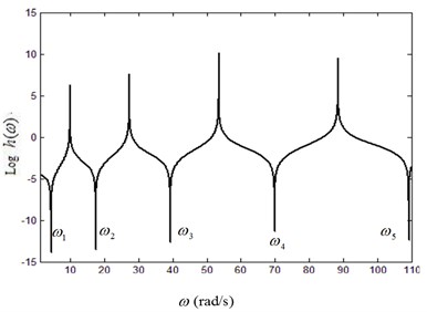
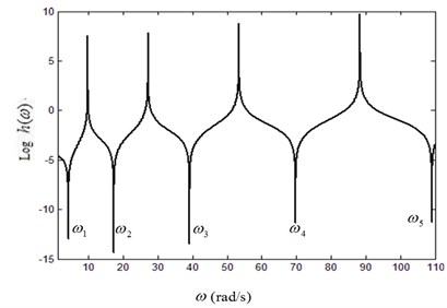
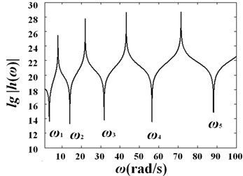
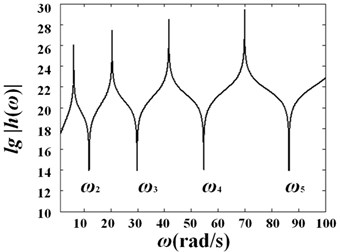
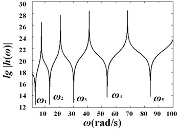
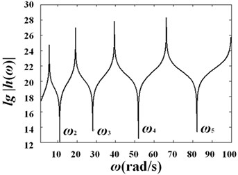
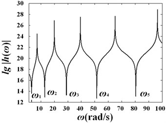
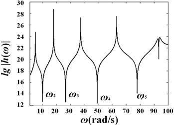
Fig. 4Curves of lg(h)-frequency under different fluid velocities: a) V=0, b) V=15 m/s, c) V=25 m/s
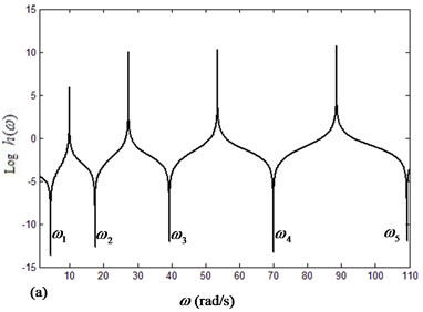
a)
b)
c)
Fig. 4 shows the curve of versus frequency under different fluid velocities, and the natural frequencies have been marked in the figure. It should be noted here that when the slope of the curve is negative infinite, the real part and the imaginary part of are both zeros. In another word, the frequencies related to the negative cuspidal points are the natural frequencies of the fluid-conveying pipe.
4.2. Variable diameter pipe conveying fluid
To simply supported variable diameter pipes conveying fluid, we choose three different diameter variation coefficients, that is 0.1, 0.2, 0.3, respectively. Given that the Yang’s modulus of the pipe material is , the outer and inner diameters of pipe at the origin of the pipe are and respectively. The pipe length is , the density of pipe material is , and the density of fluid is . The natural frequencies are computed under the following three different fluid velocities: . The results are listed in Table 2.
Table 2Natural frequencies of variable diameter pipe conveying fluid with different diameter variation coefficients under different fluid velocities
and fluid velocities | Natural frequencies | |||||
3.54 | 14.14 | 31.82 | 56.56 | 88.36 | ||
3.10 | 13.80 | 31.52 | 56.26 | 88.08 | ||
– | 11.92 | 29.84 | 54.68 | 86.54 | ||
3.34 | 13.48 | 30.32 | 53.88 | 84.18 | ||
2.88 | 13.12 | 29.98 | 53.56 | 83.88 | ||
– | 11.10 | 28.20 | 51.88 | 82.84 | ||
3.16 | 12.92 | 29.04 | 51.62 | 80.58 | ||
2.66 | 12.52 | 28.68 | 51.28 | 80.42 | ||
– | 10.30 | 26.76 | 49.44 | 77.98 | ||
From Table 2, we can find that to the same diameter variation coefficient , the natural frequencies decrease as the fluid velocity increases, and that the larger we choose, the smaller the natural frequencies we get. The results obtained above agree with that in the researches of Hannoyer and Paidoussis [8].
Additionally, we notice that when the fluid velocity reaches 25 m/s, the first order natural frequency has already vanished. So we can conclude that such velocity has already exceeded the critical velocity of the pipe. Actually, the critical velocities of variable diameter pipe conveying fluid with different diameter variation coefficients are 0.1, 0.2, ; 0.3, , respectively, as shown in Fig. 5.
Fig. 5Curves of first order natural frequency versus fluid velocity
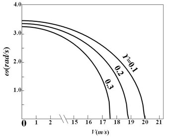
Fig. 6Buckling of the variable diameter pipe conveying fluid
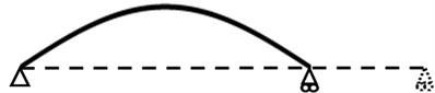
When the fluid velocity reaches the critical value, the simply supported variable diameter pipe would yield buckling, as a form of static instability, as shown in Fig. 6. Further, the instability would result in the failure of the pipe.
It is obvious that the larger the diameter variation coefficient is, the smaller the critical velocity we get, which agree with the result in the researches of Hannoyer and Paidoussis [8].
Fig. 7 shows the curves of versus frequency for variable diameter pipe conveying fluid with different diameter variation coefficients under velocity and .
Fig. 7Curves of log(h)-frequency with different diameter variation ratio under different fluid velocities: a) γ=0.1, V0=0; b) γ=0.1, V0=25 m/s; c) γ=0.2, V0=0; d) γ=0.2, V0=25 m/s; e) γ=0.3, V0=0; f) γ=0.3, V0=25 m/s
a)
b)
c)
d)
e)
f)
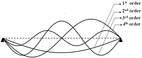
After we obtain the natural frequencies of the variable diameter pipe, the modal shapes can be obtained correspondingly. The modal shapes of variable diameter pipe conveying fluid are shown in Fig. 8 and Table 3.
Table 3Dimensionless amplitudes of the modal shape under different flow velocities
Fluid velocity | Amplitudes | |||
1st order | 2nd order | 3rd order | 4th order | |
0.22 | 0.29 | 0.21 | 0.12 | |
0.25 | 0.31 | 0.23 | 0.15 | |
0.30 | 0.35 | 0.26 | 0.18 | |
Table 3 shows that the amplitude of the modal shape increases with increasing flow velocity. This illuminate that the increasing fluid velocity can weaken the pipe stiffness.
Fig. 8The first four orders modal shapes of variable diameter pipe conveying fluid with different diameter variation coefficients under different fluid velocities
4.3. Variable diameter pipe with damping
Damping is ignored in above calculations. But in practice, damping cannot be neglected. Here we just consider the viscous damping, then the motion equation governing the vibration of the pipe is:
where the term () is the viscous damping force, which may be introduced by immersing the pipe in liquid. Suppose that 0.05, then we can calculate the natural frequencies of the variable diameter pipe. A contrast is illustrated in Fig. 9 between damping pipe and non-damping pipe (0).
Fig. 9First order natural frequencies of damping pipe and non-damping pipe with variable fluid velocity
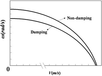
From Fig. 9, we conclude that damping would decrease the natural frequencies and critical flow velocity of the system. This has been illustrated by Paidoussis [2] in the research for a uniform fluid-conveying pipe. Moreover, damping delays the decreasing speed of natural frequency versus flow velocity. That is, as seen in Fig. 9, there is just a small difference between the two critical flow velocities, but a relatively larger difference between the natural frequencies when flow velocity is zero.
5. Conclusion
In this paper, the dynamic model was built by open system’s Hamilton’s principle on the basis of Euler-Bernoulli beam model and axial inextensible assumption. The motion equation of variable diameter pipe conveying fluid is more complex than that of uniform pipe. We employed Frobenius method to analyze the motion equation and proposed the dynamic stiffness method for free vibration analysis of variable diameter pipe conveying fluid. By using the presented method, the natural frequencies of a uniform pipe conveying fluid under different fluid velocities were obtained and the comparisons between our results and that in previous researches were made. A well agreement validates our method. The natural frequencies and modal shapes were obtained for variable diameter pipe conveying fluid with different diameter variation coefficients under different fluid velocities. We find that the natural frequencies and critical velocities of variable diameter pipe both decreased with increasing diameter variation coefficient.
References
-
Ashley H., HavilandG. Bending vibrations of a pipe line containing flowing fluid. Journal of Applied Mechanics-Transactions of the ASME, Vol. 17, Issue 3, 1950, p. 229-232.
-
Paidoussis M. P. Fluid structure interactions: slender structures and axial flow. Volume 1. London, Academic Press, 1998.
-
Doare O. Dissipation effect on local and global stability of fluid-conveying pipes. Journal of Sound and Vibration, Vol. 329, Issue 1, 2010, p. 72-83.
-
Jung D., Chung J., Mazzoleni A. Dynamic stability of a semi-circular pipe conveying harmonically oscillating fluid. Journal of Sound and Vibration, Vol. 315, Issue 1-2, 2008, p. 100-117.
-
Rinaldi S., et al. Dynamics of microscale pipes containing internal fluid flow: damping, frequency shift, and stability. Journal of Sound and Vibration, Vol. 329, Issue 8, 2010, p. 1081-1088.
-
Huang Y. M., et al. Natural frequency analysis of fluid conveying pipeline with different boundary conditions. Nuclear Engineering and Design, Vol. 240, Issue 3, 2010, p. 461-467.
-
Ragulskis M., Fedaravicius A., Ragulskis K. Harmonic balance method for FEM analysis of fluid flow in a vibrating pipe. Communications in Numerical Methods in Engineering, Vol. 22, Issue 4, 2006, p. 347-356.
-
Hannoyer M. J., Paidoussis M. P. Dynamics of slender tapered beams with internal or external axial flow 1 theory. Journal of Applied Mechanics-Transactions of the ASME, Vol. 46, Issue 1, 1979, p. 45-51.
-
Hannoyer M. J., Paidoussis M. P. Dynamics of slender tapered beams with internal or external axial flow 2 experiments. Journal of Applied Mechanics-Transactions of the ASME, Vol. 46, Issue 1, 1979, p. 52-57.
-
Arfken G. B., Weber H. J. Mathematical methods for physicists. San Diego, CA, Academic Press, 1995.
-
Housner G. W. Bending vibrations of a pipe line containing flowing fluid. Journal of Applied Mechanics-Transactions of the ASME, Vol. 19, Issue 2, 1952, p. 205-208.
About this article

This work was supported by Northwestern Polytechnical University Basic Research Fund (Grant No. JC201114) and Aeronautical Science Foundation of China (2011ZA53014).
