Abstract
Chip fault is one of the most frequently occurring damage modes in gears. Identifying different chip levels, especially for incipient chip is a challenge work in gear fault analysis. In order to classify the different gear chip levels automatically and accurately, this paper developed a fast and accurate method. In this method, features which are specially designed for gear damage detection are extracted based on a revised time synchronous averaging algorithm to character the gear conditions. Then, a modified Levenberg-Marquardt training back propagation neural network is utilized to identify the gear chip levels. In this modified neural network, damping factor and dynamic momentum are optimized simultaneously. Fisher iris data which is the machine learning public data is used to validate the performance of the improved neural network. Gear chip fault experiments were conducted and vibration signals were captured under different loads and motor speeds. Finally, the proposed methods are applied to identify the gear chip levels. The classification results of public data and gear chip fault experiment data both demonstrated that the improved neural network gets a better performance in accuracy and speed compared to the neural networks which are trained by El-Alfy’s and Norgaard’s Levenberg-Marquardt algorithm. Therefore, the proposed method is more suitable for on-line condition monitoring and fault diagnosis.
1. Introduction
In the rotating machineries, gearboxes are one of the fundamental and most important transmission parts widely used in military and industries. The main functions of these rotating machineries are achieved based on the good conditions of gearboxes. Typical applications include helicopters, wind turbines, and vehicles, etc. If faults occur in any gears of these machines during operating, serious consequences may appear. Every year, there are many helicopters crashed due to the gear faults. And for wind turbines, many unplanned downtime events are because of gear faults. This will lead to high maintenance fee and wind power lost. Therefore, effective gear faults diagnosis is crucial to prevent the mechanical system from malfunction and it can save lots of money.
Gear faults can be classified into distributed faults and localized faults. Both these fault modes can lead to catastrophic outcomes. So, many researchers paid attention to these two fault modes and did many research works. In order to diagnose gear faults automatically, many artificial intelligence and machine learning methods were used to achieve the goal. Fan and Zuo [1] improved D-S evidence theory to diagnose the faults of gearbox. Lei and Zuo [2] developed a weighted nearest neighbor classification algorithm to identify the different gear crack level. Li et al. [3] diagnosed gear faults based on adaptive wavelet packet feature extraction and relevance vector machine. Qu et al. [4] used support vector machine for both feature selection and damage degree classification of planetary gearboxes. The proposed methods exhibited the consistently effective classification both on public data and experimental data. A novel intelligent model based on wavelet support vector machine and immune genetic algorithm was proposed to diagnose the gearbox’s different fault modes [5]. In their paper, immune genetic algorithm was developed to select the optimal parameters of the wavelet support vector machine.
Besides, utilizing artificial neural networks (ANNs) for fault diagnosis is a hot research topic. In 2004, Samanta [6] reviewed fault diagnosis works using ANNs. This paper introduced the various features of ANNs systematically. Lai et al. [7] used a radial basis function network combined with cumulants to diagnose the gear faults. The cumulants were used to minimize the Gaussian noise and increase the signal-to-noise ratio. Rafiee et al. [8] proposed a new fault diagnosis procedure using a multi-layer perceptron neural network. This model was used to identify the different wear levels of gear. Then, Rafiee et al. [9] used genetic algorithm to optimize the “mother wavelet function”, “decomposition level of the signals by means of wavelet analysis”, and “number of neurons in hidden layer” which would has a good performance for wear levels identification. Li et al. [10] developed a gear fault diagnosis method based on order cepstrum and radial basis function neural network.
Good features extraction, fast and accurate classification methods are the two most important parts of automotive fault diagnosis based on artificial intelligence or machine learning methods. Some innovative works are proposed through revising feature extraction methods or classification methods. Good features which can reflect gear faults effectively are the prerequisite of fault diagnosis. Therefore, many good research works are proposed to extract the good features [11-14]. The main idea of these works is to manifest the impulsive signal produced by gear fault. Wang and Wong [11] proposed using Autoregressive (AR) model to extract the residual signal which mainly contains the impulsive signal produced by gear fault. Then, Endo and Randall [12] developed the minimum entropy deconvolution (MED) to process the residual signal extracted by AR model. MED can enable the impulse signal more impulsive which is very useful for gear fault diagnosis. Later, Yang and Makis [13] developed a new gear fault detection method based on AR model with exogenous variables. Recently, in order to overcome the deficiencies of MED, McDonald et al. [14] proposed a new impulse signal enhancement method named maximum correlated Kurtosis deconvolution (MCKD) which can extract impulsive signal more effectively than MED. In addition, time synchronous averaging (TSA) technology is often used to process the gear fault signal before other signal processing methods. And there are many statistical features developed based on the TSA [15].
When good features are available, the effectiveness of fault diagnosis depends on classification methods. In this paper, the main concern is paid to the ANNs which were widely used in fault diagnosis domain. In this field, many research works achieve the high diagnosis performance through optimizing the network parameters by various heuristic algorithms [9]. However, the training time is very long using heuristic algorithms. This is very unbeneficial to the on-line fault diagnosis which needs fast processing speed. The typical algorithm of ANN is the back-propagation algorithm, called back-propagation neural network (BPNN). Traditionally, the weights in standard BPNN are adjusted by gradient descend method according to the back propagation of error. However, Levenberg-Marquardt (LM) algorithm [16, 17] is a good combination of the Gauss-Newton technique and the steepest-descent algorithm, but avoids many of their limitations [18]. And, few works pay attention to the improvement of LM algorithm [19]. Some improved works just focus on the parameter adjustment in the LM algorithm [20-22].
In order to accelerate the learning speed and increase the fault classification accuracy for effective on-line automotive fault diagnosis, this paper addresses these problems through two methods. One is to extract more effective fault features based on a revised TSA method [23]; the other is to develop a hybrid learning algorithm to enable the ANN performing better. The main contribution and the innovation of this paper is the new gear fault diagnosis method developing based on an improved ANN learning algorithm and effective features extraction based on a revised TSA method.
The rest of this paper can be organized as follows. Section 2 introduces the improved ANN learning algorithm detail. Section 3 validates the proposed leaning algorithm using Fisher iris data. Different level gear chip faults experiments are conducted and verify the proposed fault diagnosis method in Section 4, Section 5 concludes the work.
2. Improved learning algorithm for BPNN
Gradient descend with momentum (GDM) [24] and LM algorithm [25] are the two main methods to train the network respectively.
In GDM algorithm, the weight update is related to the previous weight update. It is as follows:
where, is learning rate. is gradient which can be calculated by standard BPNN derivation process. When the weight update of input-hidden layer is calculated, is the training data . While, when the weight update of hidden-output layer is calculated, is the output of the hidden layer. is the momentum coefficient, 01.
In LM algorithm, the weight update rule is as follows:
where, the term denotes the error vector of the neural network. is the parameter which impacts convergence. If is large, the above expression approximates steepest-descent method; otherwise, the equation approximates Gauss-Newton method. is the Jacobian matrix which is defined the partial derivatives of weights for .
In GDM algorithm mentioned above, parameter is a constant. Meanwhile some papers referred to combine momentum item with LM algorithm together [21], but the merits of LM algorithm and momentum item were not exerted sufficiently. Therefore, in this paper, LM algorithm and momentum item are optimized comprehensively.
(1) Improvements on momentum item.
The form of momentum method is changed as follows:
where, could be regarded as learning rate in standard momentum method. Parameter and are dynamic. is updated according to the error alteration and previous in the former iteration. If the error reduces in this iteration, it means the previous weight update is beneficial to converge, the research direction is correct. Therefore, should be bigger for encouraging researching on this direction next time. Otherwise, should be smaller:
(2) Adjustment of .
Because can be seen as an adjuster between Gauss-Newton and Steepest-descend method. Parameter varies according to the neural network’s performance. For a given , if the error reduces, should decline to perform LM as analogous Gauss-Newton which takes advantage of fast convergence for local search. Otherwise, increases to make LM analogous Steepest-descend algorithm for searching global optima. The rule of the adjustment of is as follows:
Through the Eqs. (2)-(5), the weight update is performed by the hybrid optimization using LM algorithm and momentum method. It could search the right direction more efficiently because the weights update utilizes more information. The adjustment of makes the LM algorithm could exert the advantages of Gauss-Newton and Steepest-descend method. For traditional LM algorithm, is adjusted by 10 times increased or decreased, the too large or too small value would make the algorithm researched the optima in global or local. The algorithm may speed down or oscillate, therefore, the proposed method makes the adjustment step not too large or too small, and meanwhile, the momentum item is introduced to weaken the oscillation around the optima.
3. Validation of the proposed learning algorithm using public data
In this paper, suppose the BPNN has only one hidden layer. Hyperbolic tangent as activation function is in the hidden neurons and linear activation function in the output neurons. The number of neurons in the hidden layer is important for convergence speed. Here, empirical formula is used to decide the number of the neurons in the hidden layer:
where and are the number of the neurons in the input layer and output layer respectively. is a integer in interval [1, 10].
In this paper, the proposed learning method is validated by Fisher Iris Data. In addition, the proposed method is compared with El-Alfy’s LM (ELM) training BPNN [22] and Nørgaard’s LM (NLM) training BPNN [26]. Fisher Iris data should be normalized by “mapminmax” function provided by Matlab toolbox in advance. The maximum iteration step is 50.000.000, the training error goal is 1e-10, and the initial is 1, and the initial is 0.01.
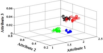
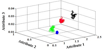
The Fisher Iris data is one of the most famous data sets for validating machine learning methods. The data set includes 3 classes of 50 instances each. These classes refer to “setosa”, “versicolor” and “virginica” which are labeled as “1”, “2” and “3” respectively. The attributes contain sepal length, sepal width, petal length and petal width. The unit is centimeter. Whole data set is separated into 2 parts; one is for training and the other for testing. In the testing set, there are 15 tuples. For the training set, the classification map in the first three attributes can be illustrated in Fig. 1.
The output of the network should be processed in order to compare with the real value. The real output of networks may be non-integral. So “round” function is used to process the real output. The compare results are shown in Table 1.
Fig. 1Classification map in the first three attributes for training set
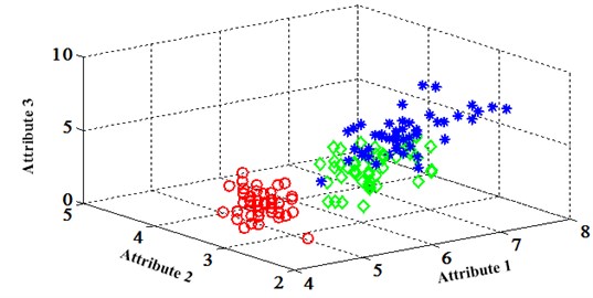
Table 1The results of different training method
Real label | Pre-processed output | Post-processed output (Predicted label) | ||||
ELM training BPNN | NLM training BPNN | Proposed LM BPNN | ELM training BPNN | NLM training BPNN | Proposed LM BPNN | |
1 | 0.9999993285 | 0.999998968 | 0.99999953 | 1 | 1 | 1 |
1 | 0.9999992952 | 0.99999965 | 0.99999953 | 1 | 1 | 1 |
1 | 0.9999993685 | 0.99999897 | 0.99999953 | 1 | 1 | 1 |
1 | 0.9999993274 | 0.999998969 | 0.99999953 | 1 | 1 | 1 |
1 | 0.9999993273 | 0.999998969 | 0.99999953 | 1 | 1 | 1 |
2 | 1.9999985480 | 31.38324967 | 2.000003934 | 2 | 31 | 2 |
2 | 2.0000023463 | 2.514282558 | 2.000001685 | 2 | 3 | 2 |
2 | 1.9999633692 | –0.86908966 | 2.002109564 | 2 | –1 | 2 |
2 | 2.0000021698 | 1.998075311 | 2.000011895 | 2 | 2 | 2 |
2 | 2.00000623203 | 1.809125959 | 2.001934675 | 2 | 2 | 2 |
3 | 2.99999644211 | 2.999999999 | 3.00000059 | 3 | 3 | 3 |
3 | 2.49818367950 | 1.999987829 | 2.506053409 | 2 | 2 | 3 |
3 | 2.99037580647 | 2.999887007 | 2.999991968 | 3 | 3 | 3 |
3 | 3.00000291431 | 2.999999992 | 3.00000059 | 3 | 3 | 3 |
3 | 2.99662415041 | 2.995428876 | 2.795373631 | 3 | 3 | 3 |
Fig. 2Classification errors represented in 2-D plane for Fisher Iris data
a) ELM training BPNN
b) NLM training BPNN
c) Proposed LM-BPNN
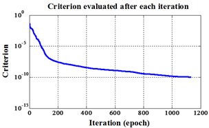
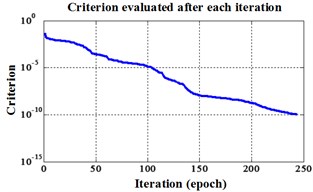
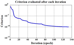
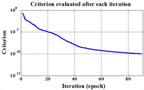
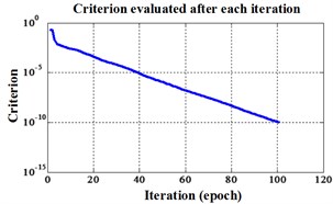
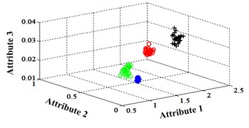
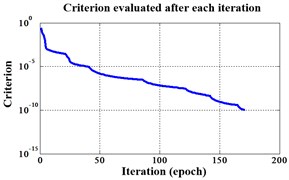
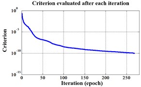
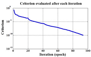
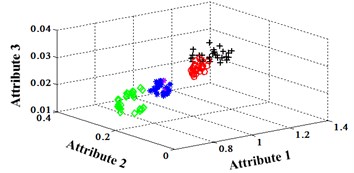
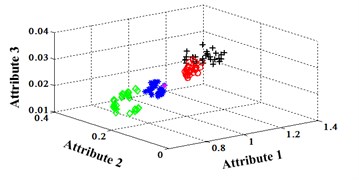
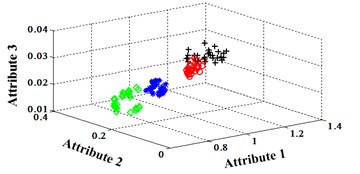
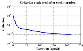
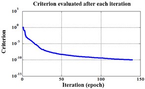
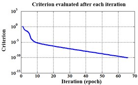
The classification errors in 2-D plane and its 3-D map in the first three attributes can be shown in Fig. 2 and Fig. 3. In the 3-D figures, the points with pink color are the wrong classification. The errors of iteration process are shown in Fig. 4.
The iteration steps, iteration time and classification accuracy are listed in Table 2.
Fig. 3Classification errors mapped in the first three attributes for Fisher Iris data
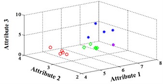
a) ELM training BPNN
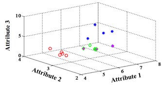
b) NLM training BPNN
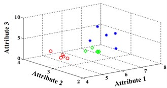
c) Proposed LM-BPNN
Fig. 4Errors of iteration process for Fisher Iris data
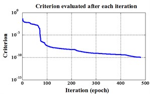
a) ELM training BPNN
b) NLM training BPNN
c) Proposed LM-BPNN
Table 2Comparison of different improved algorithms on benchmark data sets for Fisher Iris data
BPNN type | Iteration steps | Iteration time | Accuracy rate |
ELM training BPNN | 483 | 1.092726 seconds. | 93.33 % |
NLM training BPNN | 1133 | 2.337680 seconds | 73.33 % |
Proposed LM BPNN | 244 | 0.599163 seconds | 100 % |
From Fisher Iris data classification results, the proposed method is superior to other two improved BPNNs both in speed and classification accuracy. It needs only half steps and operation time compared to the ELM training BPNN. And only a quarter of steps and operation time compared to the NLM training BPNN. Besides of the speed, it can achieve 100 % accuracy.
4. Gear chip fault diagnosis using improved BPNN
4.1. Experiment setup
In order to further validate the effectiveness of proposed fault diagnosis method based on improved BPNN. A different levels gear chip fault experiment was implemented. The system includes a gearbox, a 4 kW three phase asynchronous motor for driving the gearbox, and a magnetic powder brake for loading. The speed is controlled by an electromagnetic speed-adjustable motor, which allows the tested gear to operate under various speeds. The load is provided by the magnetic powder brake connected to the output shaft and the torque can be adjusted by a brake controller.
The data acquisition system is composed of acceleration transducers, PXI-1031 mainframe, PXI-4472B data acquisition cards, and LabVIEW software. The type of transducers is 3056B4 of Dytran Company. There are four transducers which are mounted in different places on gearbox. In order to acquire the speed and torque information, a speed and torque transducer is installed in the input shaft as illustrated in Fig. 5. For this transducer, one revolution of input shaft will produce 60 impulses.
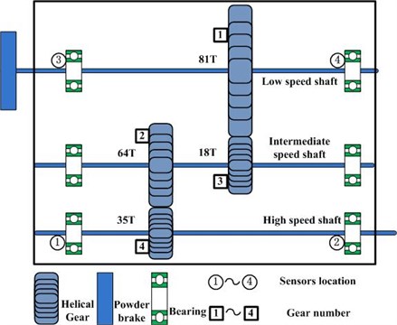
As shown in Fig. 6, the gearbox has three shafts, which are mounted to the gearbox housing by rolling element bearings. Gear 1 on low speed (LS) shaft has 81 teeth and meshes with gear 3 with 18 teeth. Gear 2 on intermediate speed (IS) shaft has 64 teeth and meshes with gear 4, which is on the high speed (HS) shaft and has 35 teeth. There are four transducers are mounted on the gearbox as depicted in Fig. 6 using circle.
Fig. 5Test-rig of gearbox
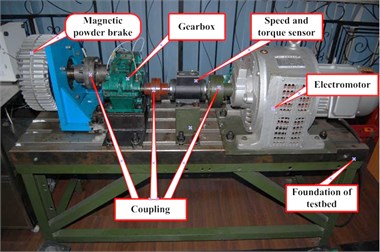
Fig. 6Structure of gearbox and the transducers location
The chip faults are implanted on one tooth of gear 2 which meshes with gear 4 on HS shaft. The chip widths are 2 mm, 5 mm, and 10 mm respectively. It can be depicted in Fig. 7. They were tested under three different loads and rotating speeds. The rotating speeds are about 800 rpm, 1.000 rpm and 1.200 rpm. The loads are 10 N·m, 15 N·m, and 20 N·m. For every chip fault level and operating condition, 60 data samples are acquired. In this paper, the data sets under 1.200 rpm and three different loads are used to validate the proposed methods. The signals collected by sensor 1 are used for feature extraction and model validation.
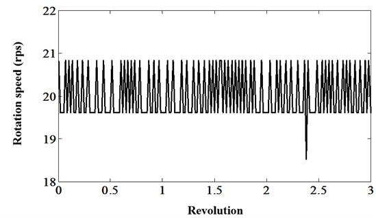
TSA can be used for shaft and gear analysis to both control variation in shaft speed and to reduce non-synchronous noise. Many statistical features specially developed for gear damage detection are based on TSA processing [15]. However, traditional TSA techniques suppose the rate of change in the shaft under analysis is linearity. In real, because of the varying load, the rate of change of the shaft changes more than 10 times in one revolution as shown in Fig. 8.
The multiple changes in sign of the derivative of the shaft speed will has a bad effect on gear fault analysis. In order to address this problem, Bechhoefer [23] proposed a revised TSA technique which can capture the speed variation in one revolution. Based on this new TSA technology, eight features are extracted for different chip levels identification. They are FM0, FM4, FM4*, NA4, NB4, ER (energy ration), M6A, and M8A. After the feature extraction, the proposed BPNN can be used to classify the different chip level.
Fig. 7Three different levels chip tooth
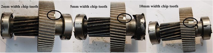
Fig. 8The rotation speed variation in three revolutions
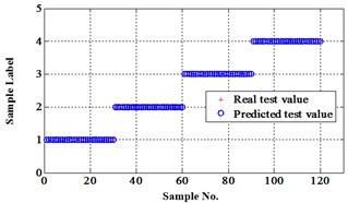
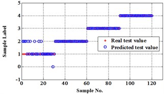
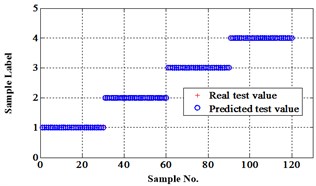
4.2. Results under operation condition 1.200 rpm and 20 N·m
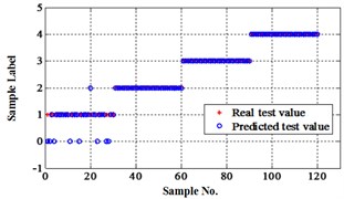
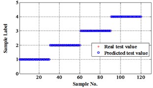
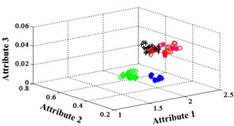
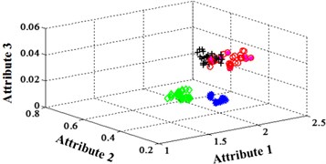
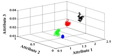
Before the data analysis, it states that all the initial parameters of proposed methods are same as used in Fisher Iris data. There are four degradation states for this chip faults experiment. They are normal, slight chip (2 mm width chip), medium chip (5 mm width chip), and severe chip (10 mm width chip). These four states can be denoted as ‘1’, ‘2’, ‘3’, and ‘4’ labels. 60 signal samples were collected for each state. After fault features extraction, 30 feature samples from each state are used for training, the rest are for testing. The classification map in the first three attributes of data under operation condition 1.200 rpm and 20 N·m can be depicted in Fig. 9.
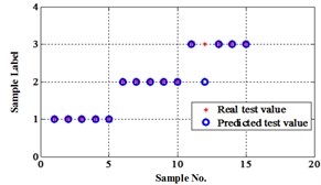
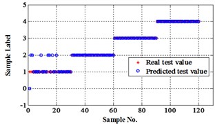
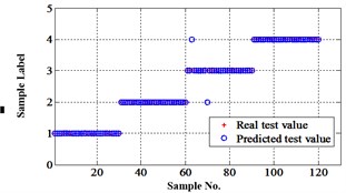
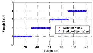
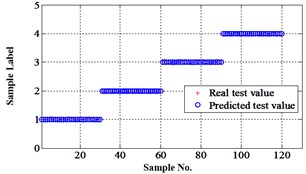
The compared outputs of different networks are operated by “round” function. Because the limited pages and amount of data, the results are not shown in this paper. Similar to the public data validation, the classification errors in 2-D plane and its 3-D map in the first three attributes can be shown in Fig. 10 and Fig. 11. In the 3-D figures, the points with pink color are the wrong classification. The errors of iteration process are shown in the Fig. 12.
The iteration steps, iteration time and classification accuracy are listed in Table 3.
Table 3Comparison of different neural networks under operation condition 1.200 rpm and 20 N·m
BPNN type | Iteration steps | Iteration time | Accuracy rate |
ELM training BPNN | 133 | 0.421206 seconds. | 93.33 % |
NLM training BPNN | 90 | 0.333872 seconds. | 92.5 % |
Proposed LM BPNN | 101 | 0.283346 seconds. | 100 % |
Fig. 9Classification map in the first three attributes of the signals under operation condition 1.200 rpm and 20 N·m
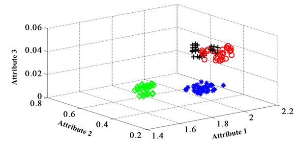
Fig. 10Classification errors in 2-D of the signals under operation condition 1.200 rpm and 20 N·m
a) ELM training BPNN
b) NLM training BPNN
c) Proposed LM-BPNN
Fig. 11Classification errors mapping in the first three attributes of the signals under operation condition 1.200 rpm and 20 N·m
a) ELM training BPNN
b) NLM training BPNN
c) Proposed LM-BPNN
Fig. 12Errors of iteration process of the signals under operation condition 1.200 rpm and 20 N·m
a) ELM training BPNN
b) NLM training BPNN
c) Proposed LM-BPNN
4.3. Results under operation condition 1.200 rpm and 15 N·m
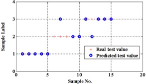
Similar to the chip fault classification under operation condition 1.200 rpm and 20 N·m, 30 fault samples are used for training and the rest are for testing. Classification errors in 2-D plane and its 3-D map in the first three attributes can be shown in Fig. 13 and Fig. 14. Similarly, the points with pink color are the wrong classification. The errors of iteration process are shown in the Fig. 15.
The iteration steps, iteration time and classification accuracy are listed in Table 4.
Table 4Comparison of different neural networks under operation condition 1.200 rpm and 15 N·m
BPNN Type | Iteration steps | Iteration time | Accuracy rate |
ELM training BPNN | 171 | 0.551402 seconds. | 100 % |
NLM training BPNN | 269 | 0.670372 seconds. | 91.67 % |
Proposed LM BPNN | 94 | 0.460250 seconds. | 100 % |
Fig. 13Classification errors in 2-D of the signals under operation condition 1.200 rpm and 15 N·m
a) ELM training BPNN
b) NLM training BPNN
c) Proposed LM-BPNN
Fig. 14Classification errors mapping in the first three attributes of the signals under operation condition 1.200 rpm and 15 N·m
a) ELM training BPNN
b) NLM training BPNN
c) Proposed LM-BPNN
Fig. 15Errors of iteration process of the signals under operation condition 1.200 rpm and 15 N·m
a) ELM training BPNN
b) NLM training BPNN
c) Proposed LM-BPNN
4.4. Results under operation condition 1.200 rpm and 10 N·m
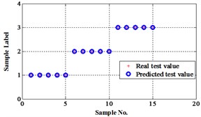
Similarly, classification errors in 2-D plane and its 3-D map in the first three attributes can be shown in Fig. 16 and Fig. 17. The points with pink color are the wrong classification. The errors of iteration process are shown in the Fig. 18.
The iteration steps, iteration time and classification accuracy are listed in Table 5.
Table 5Comparison of different neural networks under operation condition 1.200 rpm and 10 N·m
BPNN type | Iteration steps | Iteration time | Accuracy rate |
ELM training BPNN | 213 | 0.732871 seconds. | 98.33 % |
NLM training BPNN | 140 | 0.524008 seconds. | 99.17 % |
Proposed LM BPNN | 66 | 0.249918 seconds. | 100 % |
From the gear chip fault level classification results, we can see that the proposed method is faster and has better classification accuracy than the other two improved LM BPNN. The proposed method also achieves 100 % gear fault level identification accuracy. So, it can be concluded that the proposed method can be used for on-line fault diagnosis and will be very effective for identifying different fault level.
However, there are three issues waiting for our further deep research in future to achieve the application goal. They are: (1) The initial is very important. It impacts the training speed and accuracy of the network. We tested different and found that too big or too small the initial is, the training process is time-taking and hard to calculate. Especially, the Hessian vector is hard to be calculated. So how to select the initial parameter adaptively is valuable. (2) By reviewing the existed literatures, we found most publications stress the parameter should be bigger or smaller by certain step like the learning rate in the standard BPNN. Similarly, the fix adjustment of may not balance the Gauss-Newton and Steepest descend very well. So, we will focus on how to adjust in the training process and make a better performance. (3) When there are several faults existing simultaneously, how to use proposed method to diagnose the different fault?
Fig. 16Classification errors in 2-D of the signals under operation condition 1.200 rpm and 10 N·m
a) ELM training BPNN
b) NLM training BPNN
c) Proposed LM-BPNN
Fig. 17Classification errors mapping in the first three attributes of the signals under operation condition 1.200 rpm and 10 N·m
a) ELM training BPNN
b) NLM training BPNN
c) Proposed LM-BPNN
Fig. 18Errors of iteration process of the signals under operation condition 1.200 rpm and 10 N·m
a) ELM training BPNN
b) NLM training BPNN
c) Proposed LM-BPNN
5. Conclusions
A new gear fault diagnosis method based on an improved training algorithm BPNN is proposed in this paper. The LM jointed with the momentum item is optimized simultaneously for training BPNN. This new algorithm can have faster operation speed and achieve better classification accuracy compared to two other improved LM algorithms. Firstly, this proposed method is validated using Fisher iris data. Then, it is used to diagnose the different gear chip fault level under three different operation conditions. All the results from public data and experimental data verified that the proposed method has better accuracy performance and can complete the calculation work rapidly. Therefore, this method is very suitable for on-line automotive gear fault diagnosis. This will be meaningful and will save maintenance money and downtime cost greatly. In addition, using this new method to diagnose the multi-faults of gearbox needs to be researched in future.
References
-
Fan X. F., Zuo M. J. Fault diagnosis of machines based on D-S evidence theory. Part 2: Application of the improved D-S evidence theory in gearbox fault diagnosis. Pattern Recognition Letters, Vol. 27, Issue 5, 2006, p. 377-385.
-
Lei Y. G., Zuo M. J. Gear crack level identification based on weighted K nearest neighbor classification algorithm. Mechanical Systems and Signal Processing, Vol. 23, Issue 5, 2009, p. 1535-1547.
-
Li N., Liu C., He C., Li Y., Zha X. F. Gear fault detection based on adaptive wavelet packet feature extraction and relevance vector machine. Journal of Mechanical Engineering Science, Vol. 225, Issue 11, 2011, p. 2727-2738.
-
Qu J., Liu Z., Zuo M. J., Huang H. Z. Feature selection for damage degree classification of planetary gearboxes using support vector machine. Journal of Mechanical Engineering Science, Vol. 225, Issue 9, 2011, p. 2250-2264.
-
Chen F. F., Tang B. P., Chen R. X. A noval fault diagnosis model for gearbox based on wavelet support vector machine with immune genetic algorithm. Measurement, Vol. 46, Issue 8, 2013, p. 220-232.
-
Samanta B. Artificial neural networks and genetic algorithms for gear fault detection. Mechanical Systems and Signal Processing, Vol. 18, Issue 5, 2004, p. 1273-1282.
-
Lai W. X., Tse P. W., Zhang G. C., Shi T. L. Classification of gear faults using cumulants and the radial basis function network. Mechanical Systems and Signal Processing, Vol. 18, Issue 2, 2004, p. 381-389.
-
Rafiee J., Arvani F., Harifi A., Sadeghi M. H. Intelligent condition monitoring of a gearbox using artificial neural network. Mechanical Systems and Signal Processing, Vol. 21, Issue 4, 2007, p. 1746-1754.
-
Rafiee J., Tse P. W., Harifi A., Sadeghi M. H. A novel technique for selecting mother wavelet function using an intelligent fault diagnosis system. Expert Systems with Applications, Vol. 36, Issue 3, 2009, p. 4862-4875.
-
Li H., Zhang Y. P., Zheng H. Q. Gear fault detection and diagnosis under speed-up condition based on order cepstrum and radial basis function neural network. Journal of Mechanical Science and Technology, Vol. 23, Issue 10, 2009, p. 2780-2789.
-
Wang W., Wong A. K. Autoregressive model-based gear shaft fault diagnosis. Journal of Vibration and Acoustics, Vol. 124, Issue 2, 2002, p. 172-179.
-
Endo H., Randall R. Enhancement of autoregressive model based gear tooth fault detection by the use of minimum entropy deconvolution filter. Mechanical Systems and Signal Processing, Vol. 21, Issue 2, 2007, p. 906-919.
-
Yang M., Markis V. Arx model-based gearbox fault detection and localization under varying load conditions. Journal of Sound and Vibration, Vol. 329, Issue 24, 2010, p. 5209-5221.
-
McDonald G. L., Zhao Q., Zuo M. J. Maximum correlated Kurtosis deconvolution and application on gear tooth chip fault detection. Mechanical Systems and Signal Processing, Vol. 33, 2012, p. 237-255.
-
Samuel P. D., Pines D. J. A review of vibration-based techniques for helicopter transmission diagnostics. Journal of Sound and Vibration, Vol. 282, Issue 1-2, 2005, p. 475-508.
-
Castillo E., Fontenla-Romero O., Guijarro-Berdiñas B., Alonso-Betanzos A. A global optimum approach for one-layer neural networks. Neural Computation, Vol. 14, Issue 6, 2002, p. 1429-1449.
-
Güler I., Übeyli E. D. A recurrent neural network classifier for Doppler ultrasound blood flow signals. Pattern Recognition Letters, Vol. 27, Issue 13, 2006, p. 1560-1571.
-
Übeyli E. D., Güler I. Spectral analysis of internal carotid arterial Doppler signals using FFT, AR, MA, and ARMA methods. Computers in Biology and Medicine, Vol. 34, Issue 4, 2004, p. 293-306.
-
Nguyen G. H., Bouzerdoum A., Phung S. L. A supervised learning approach for imbalanced data sets. 19th International Conference on Pattern Recognition, Tampa, 2008, p. 1-4.
-
Ling M. Q., Liu W. W. Research on intrusion detection systems based on Levenberg-Marquardt algorithm. International Conference on Machine Learning and Cybernetics, Kunming, Vol. 7, 2008, p. 3684-3688.
-
Wang X. P., Huang Y. S. Predicting risks of capital flow using artificial neural network and Levenberg Marquardt algorithm. International Conference on Machine Learning and Cybernetics, Kunming, Vol. 3, 2008, p. 1353-1357.
-
El-Alfy E. S. M. Detecting pixel-value differencing steganography using Levenberg-Marquardt neural network. IEEE Symposium on Computational Intelligence and Data Mining, Singapore, 2013, p. 160-165.
-
Bechhoefer E. An enhanced synchronous averaging for rotating equipment analysis. MFPT Conference, Cleveland, 2013, p. 1-10.
-
Phansalkar V. V., Sastry P. S. Analysis of the back-propagation algorithm with momentum. IEEE Transactions on Neural Networks, Vol. 5, Issue 3, 1994, p. 505-506.
-
Marquardt D. W. An algorithm for least-squares estimation of non-linear parameters. Journal of the Society of Industrial and Applied Mathematics, Vol. 11, Issue 2, 1963, p. 431-441.
-
Norgaard M. Neural network based system identification toolbox. Tech. Report. 00-E-891, Department of Automation, Technical University of Denmark, 2000.
About this article

The authors would like to thank anonymous referees for their remarkable comments and great support by Key Project supported by National Science Foundation of China (51035008); Natural Science Foundation Project of Chongqing (CSTC, 2009BB3365), and the Fundamental Research Funds for the State Key Laboratory of Mechanical Transmission, Chongqing University (SKLMT-ZZKT-2012 MS 02).
