A Bayesian approach for seismic recurrence parameters estimation

Khanzadi, Mostafa; Nicknam, Ahmad; Yazdani, Azad; Motaghed, Sasan

Journal of Vibroengineering

Browse Journal

Submit article

Published: 31 March 2014

Check for updates

A Bayesian approach for seismic recurrence parameters estimation

Mostafa Khanzadi¹

Ahmad Nicknam²

Azad Yazdani³

Sasan Motaghed⁴

^{1, 2, 4}School of Civil Engineering, Iran University of Science and Technology, P. O. Box 16765-163, Tehran, Iran

³Department of Civil Engineering, University of Kurdistan, P. O. Box 416, Sanandaj, Iran

Corresponding Author:

Mostafa Khanzadi

Cite the article Download PDF

Downloads 1273

Abstract

Recurrence models apply historical seismicity information to seismic hazard analysis. These models that play an important role in the obtained hazard curve are determined by their parameters. Recurrence parameters estimation has some features that lie in missing-data problems category. Thus, the observed data cannot be used directly to estimate model parameters. Furthermore discussion about results reliability and probable conservatism is impossible. The present study aims at offering an approach for Gutenberg-Richter parameters ( $a$ and $b$ -values) estimation and determine their variation. Applying the proposed method to analyses of the heterogeneous data sets of seismic catalog, one would calculate valid estimates for recurrence parameters. This method has the capability to reflect all known sources of variability. The results of the case study clearly demonstrate applicability and efficiency of the proposed method, which can easily be implemented not only in advanced but also in practical seismic hazard analyses.

1. Introduction

Probabilistic seismic hazard analysis (PSHA) aims at providing unbiased estimation of seismic hazard in future time period [1]. For reliable estimation and safe design platform preparation [2, 3], PSHA should consider uncertainties and randomness in size, location and recurrence of earthquakes. Recurrence law describes the distribution of earthquake size in a given period of time. One of the fundamental assumptions of PSHA is that the recurrence law obtained from the past seismicity is fit to the future seismicity. Hence, seismicity parameters like $m_{m a x}$ and recurrence parameters play an important role in PSHA. This is why the wide and polemical discussions about the recurrence models (Gutenberg and Richter distribution (G-R law) vs. independent rates in every magnitude), magnitude scales and bins, and the fitting algorithm (least squares (LS) or maximum likelihood (ML)) [4]. Dong et al. presented a method for recurrence relationship development which is compatible with the geological, historical, and instrumental data based on the maximum entropy principle. They also suggested a modified maximum entropy principle method to incorporate long-term geological information of large earthquakes with the short-term historical or instrumental information of small to medium-size earthquakes [5]. In another paper, Dong et al. show why the empirical method using only short historical earthquake data cannot obtain reliable hazard estimation. They developed the Bayesian framework to use the energy flux concept, seismic moment and geological observation in the seismic hazard analysis [6]. Kijko and sellevoll use the maximum likelihood estimation of earthquake hazard parameters (which previously had been used by aki [7]) from incomplete data files [8]. This method has been used extensively in the PSHA. Lamarre et al. described a methodology to assess the uncertainty in seismic hazard estimates. They use a variant of the bootstrap statistical method to combine the uncertainty due to earthquake catalog incompleteness, earthquake magnitude, and recurrence and attenuation models [9]. Turnbull and Parsons use Gumbel plotting of historical annual extreme earthquake magnitudes and Monte Carlo method for determining earthquake recurrence parameters respectively [10, 11].

In this study, we present a simple alternative method for Gutenberg-Richter (G-R) law parameters ( $a$ and $b$ -values) estimation based on the assumption of seismicity stationarity. The key feature of the method is the correction of the catalog heterogeneity through the use of Bayes’ formulation. So, it is possible to utilize the entire earthquake catalog in a region and estimate the uncertainties in seismicity parameters using the bootstrap statistic method. The proposed method is assessed as a simple method that also gives uncertainties resulting from estimation method. To illustrate the effect of the method on hazard computation, we give recurrence parameters for Tehran metropolitan as an example.

2. G-R law parameters estimation

Gutenberg-Richter law for earthquake recurrence is expressed as [12]:

1

l o g [N (M)] = a - b M,

where $M$ denotes magnitude, $N$ is the number of events with magnitude not less than $M$ , and $a$ and $b$ are constant coefficients. It is supposed that seismic sources have a maximum earthquake magnitude, $m_{m a x}$ , which cannot be exceeded. Also for engineering purposes, the effects of small earthquakes that are not capable of causing significant damage are of little interest. Therefore earthquakes with magnitude smaller than a specified threshold magnitude, $m_{m i n}$ , or larger than $m_{m a x}$ are removed and the Eq. (1) can be written as:

2

f_{M} (m) = k β e^{- β (m - m_{m i n})}, m_{m i n} \leq m \leq m_{m a x},

k = {[1 - e^{- β (m_{m a x} - m_{m i n})}]}^{- 1},

where $β = b ln 10$ . Eq. (2) is called bounded G-R recurrence law or double truncated G-R law. Eqs. (1) and (2) parameters are calculated using LS or ML method based on seismic catalog data regression.

For reliable regression and parameters determination, homogeneity of the data is very important issue. Spatial and temporal changes in seismic event record system which provide data for future processing, construct problematic structure for analysis. Regarding the non-homogeneous nature of the data in seismic catalos, any estimation approach should satisfy data homogeneity. Homogeneity assurance is possible in two ways: employing only fairly complete recent catalog data (e.g., recent 50 years) that homogeneity is surly satisfied, and utilizing the entire catalog data and homogenize it. Each method suffers from major drawbacks. For example, in the first method the time period of instrumental data is usually shorter than the recurrence rate of large earthquakes, while, large earthquake can influences the estimated parameters strongly. Therefore, the major part of the seismicity information is omitted and results are not valid. The main source of non-homogeneity of seismic catalog is different magnitude scales, existence of the aftershocks and catalog incompleteness. Catalog incompleteness results from incompleteness earthquake reporting due to the ill record system i.e. weak detection capability, noise induced problems, and overlapping of seismograms in high activity seismic region [13].

Catalog incompleteness means the existence of missing earthquakes that need to be covered in any subsequent processing. Finding the sophisticated method for seismic catalog processing, remove its heterogeneity and convert it to the homogeny catalog to be suitable for seismicity parameters estimation is considered in section 3.

3. Methodology

In this section, we describe a new approach for the reliable seismicity parameters estimation based on the most probable entire seismic catalog data. This approach employs some statistical tools namely stochastic processes, missing data theory, Bayes’ theorem and bootstrap sampling method. We modify the seismic catalog to cover the entire recorded and unrecorded (but likely to occur) earthquakes in a region. In this process the reported real data remains unchanged in the catalog (weighted by one) while those likely to happen (missing data) are weighted by their occurrence probability value. In other words, we append new earthquakes to the existing catalog, which are probably happened but are not recorded (i.e., missing earthquakes).

In the proposed methodology, for catalog completion and $a$ and $b$ values estimation, it is essential to determine the degree of catalog incompleteness. We know that the catalog recording properties are not constant in the entire time span, i.e., any scientific, technical, economic and social growth can change recording precision. So, catalog completeness properties are non uniform and it is necessary to determine magnitude bounds of catalog with uniform recording properties. Afterward it is possible to complete catalog in the incomplete parts regarding their degrees of incompleteness.

3.1. Completeness regions determination

Completeness region (CR) refers to a certain geographical region, magnitude range and time period where the detection probability is homogeneous [9].

Most PSHA methods consider earthquakes as stationary processes (i.e., time invariant over a long period), and estimate future seismicity rate directly from the past information [14]. A stationary process is defined as a stochastic process whose means, variance and covariance are considered to be constant in time. In stationarity investigations, space, magnitude and time ranges are critical issues. Therefore, in a specified region, we select magnitude ranges and time period in a manner that stationarity can be satisfied.

Magnitude range is the smallest range where stationarity is met. It should be small enough to best provide homogeneity. It is not necessary for magnitude ranges to be equal to each other. In regions with moderate seismicity, where the earthquake of upper magnitude is rare, sometimes it is useful to enlarge ranges with magnitude.

Geographical region should be considered as the largest area where recording homogeneity can be assumed. The geographical region enlargement can provide possibility to satisfy stationarity in smaller magnitude ranges. Usually, geographical region is given.

The time period is determined based on the homogeneity of the recording in each range. Therefore, all the factors that affect the ability of recording play role in the determination of homogenous time periods. As a result, time intervals can be determined as the time between important changes of the aforementioned factors. Alternatively, considering the impact of these factors on the completeness magnitude ( $M_{c}$ ) and its high sensitivity, time periods can be determined as the intervals between $M_{c}$ changes. The advantage of this alternative approach is that time periods of $M_{c}$ changes are usually available from other studies.

It should be noted that aftershocks are removed from the catalog because the current methods of catalog completeness test are based on power law (G-R), which in turn, it is based on the presumption of linear behavior of earthquakes in magnitude domain.

3.2. Catalog completion and parameters estimation

For catalog completion, it is necessary to find missing earthquakes and adding them to the catalog. We use a statistical approach to discover probable earthquake. Firstly, we introduce some preliminary definitions.

Record ratio ( $R R$ ) is defined as the ratio of $n_{C R} (t, g, m)$ to the $n_{C C R} (t_{c}, g, m)$ , where $n_{C R} (t, g, m)$ is the record rate in a given completeness region (geographical region ( $g$ ), magnitude range ( $m$ ) and time period ( $t$ )) and $n_{C C R} (t_{c}, g, m)$ is the record rate for the same geographical region ( $g$ ) and magnitude range ( $m$ ) but for the time period of complete catalog ( $t_{c}$ ). Complete catalog completeness region ( $C C C R$ ) refers to the recent completeness region.

$n_{C R} (t, g, m)$ is equal to ( $N_{C R} (t, g, m) / t$ ), where $N_{C R} (t_{c}, g, m)$ is the number of earthquakes in a given completeness region and $n_{C C R} (t_{c}, g, m)$ is achieved form the same approach for $C C C R$ s ( $n_{C C R} (t_{c}, g, m) = (N C C R (t_{c}, g, m) / t_{c}$ ) where $N_{C C R} (t_{c}, g, m)$ is the number of earthquakes in $C C C R$ s). Notably, there is a one to one relationship between records and events in $C C C R$ s.

Recorded probability ( $R P_{C R (t, g, m)}$ ) is defined as the chance of recording and/or reporting the occurred earthquake in a catalog and is determined from $R R$ using the negative binomial distribution [9]. The time interval recorded probability ( $T I R P$ ) in the time period between the two predefined time intervals denoted by ( $T$ ) is calculated by Eq. (3) expressed as:

3

T I R P_{T g m} = {(R P_{C R (t, g, m)})}^{T / t} .

Since $T I R P$ is defined based on the occurrence ratio, it can be regarded as conditional $T I R P$ and denoted as:

4

T I R P_{T g m} = p_{T, g, m} (\frac{A}{B}),

where, $A$ and $B$ stand for earthquake recording and occurrence probabilities respectively. Afterwards for simplicity we omit the subscripts and write ( $p (A / B)$ ) instead of ( $p_{T, g, m} (A / B)$ ).

Detection probability is defined as the probability of existence unrecorded events in completeness region between two successive main events and calculated as complementary probability of the RR in the following form:

5

P (\frac{A^{'}}{B}) = 1 - p (\frac{A}{B}),

where $A'$ denotes detection probability.

Earthquake scenario is defined as a set of probable earthquake between two recorded earthquakes and evidently respective in catalog after removing clusters, duplicates and magnitude scale conversion. Due to the lack of a certain report of these scenarios, it is necessary to determine their occurrence probabilities quantitatively. The basic idea of the propose method is catalog adjustment. Adjustment is any process that corrects the records based on estimated recoding error [15]. Having the above definition, we can generate probable missing data and complete the catalog with probable sets of earthquakes. This catalog contains all plausible scenarios for earthquake occurrence and we call it plausible catalog. To calculate the scenarios probability, occurrence probability conditional on detection probability should be calculated. If $P (B / A')$ is occurrence probability conditional on event detection, $P (B' / A')$ is non occurrence probability conditional on event detection and $B'$ denotes non occurrence probability. According to Bayes’ theorem, $P (B / A')$ is obtained from the Eq. (6) as:

6

P (\frac{B}{A^{'}}) = {(1 - \frac{1}{P (\frac{A^{'}}{B})} + \frac{1}{P (B) P (\frac{A^{'}}{B})})}^{- 1} .

Thus, to determine $P (B / A')$ , detection probability $P (A' / B)$ and occurrence probability $P (B)$ are required. The detection probability is already obtained and occurrence probability can be derived based on the following argument: To define record probability, the earthquake annual rate in the completeness region (in the completed part of the catalog) divides by the annual rate of earthquake in the recent time period of that completeness region (complete part of the catalog). It is implied that the annual rate of earthquake in the complete part of the catalog is known as the annual earthquake rate. Assuming Poisson distribution, we can determine the probability of earthquake occurrence between two consecutive earthquakes:

7

P (B) = P (n; v) = \frac{e^{- v} v^{n}}{n!},

where $n$ is the number of missing earthquakes and $ν$ is earthquake rate within the time period between two consecutive earthquakes which is equal to annual earthquake rate multiplied by the number of years between two consecutive earthquakes.

Having the two probabilities of $P (A' / B)$ and $P (B)$ , we can calculate $P (B / A')$ and the occurrence probabilities for each scenario. Now we add some sets of earthquakes and their occurrence probabilities between each pair of consecutive earthquakes. So, plausible catalog contain recorded earthquakes (weighted by 1) and added earthquakes (weighted according the above method). For catalog completion with $m_{1}$ initial main events, ( $m_{1} - 1$ ) samples of the ( $m_{1} - 1$ ) added earthquakes sets (a member from each set) should be attached to the initial catalog in each magnitude range. These samples display the numbers of missing earthquakes in time periods between main events. The events have unequal weights, so they cannot have equal roles in regression. This problem is solved by using bootstrap weighted sampling. In this method sampling is done by the replacement from the initial set [16]. Bootstrap samples include events that might be occurred, not actually occurred. Each of the $m_{1} - 1$ initial sets has $n$ members, which are used to produce $D$ bootstrap duplicates each with $m_{1} - 1$ members. $D$ represents big number like 10000 or more. For each of the $n$ earthquake numbers in the $m_{1} - 1$ added sets, the chance of existence a particular member in the bootstrap duplicates is determined by generating random number between 0.0 and 1.0. Each of the bootstrap duplicates and initial catalog construct a completed catalog. So, we generate $D$ completed catalog. $a$ and $b$ -values for each of these catalogs are estimated, using ML Regression analysis. Therefore, a $D$ -member set is made for each parameter and we can calculate the mean and standard deviation of $a$ and $b$ values.

4. Case study and discussion

The proposed approach here is implemented for Tehran city, the capital of Iran, as an example. Then, the recurrence model parameters are compared with those of a previous works. The existence of the active faults (like North Tehran, Mosha, Pishva, North Ray, South Ray, Garmsar and Kahrizak), the alluvium deposits of Tehran plain, and the destructive earthquakes occurrence, all clarify the seismicity of this region. Estimation the seismicity parameters of this region are the subject of many studies. The results of some previous works are shown in Table 1. Clearly, the results are dissimilar. The main reasons for the observed differences are catalog, $m_{m i n}$ and magnitude scale differences as well as different declustering, data preparation, and estimation methods.

Table 1G-R relation parameters proposed by some researchers for Tehran and its vicinity

Refrences	Time period	$a$ -value	$b$ -value	Magniude
Nowroozi and Ahmdi [17]	1900-1976, $M_{w} >$ 5.9 1960-1976, $M_{w} <$ 5.9	3.69	0.77	$M_{w}$
Niazi and Bozorgnia [18]	before 1990	–	0.85±0.05	$M_{b} \geq$ 4
Jafari [19]	1996-2007	5.09	0.91±0.07	$M_{n} \geq$ 2.5
Ghodrati et al. [20]	after 1900	2.29	0.63	$M_{s} \geq$ 4
	before1900	1.25	1.04
	Total	2.34	0.71

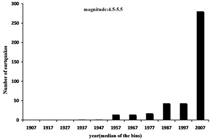
An overview of the earthquake catalog of Tehran shows its sparseness and heterogeneity. In other words, the historical data is very rare, with few exceptions. In regions where the seismogenic progress is relatively unknown, the earthquake data is sparse. In this condition, instrumental data is often integrated with paleoseismological data to cover the longer duration. Thus, the data is inconsistent. Fig. 1 shows example of non-homogeneous data in Tehran. This figure contains histogram of the earthquakes reported in each decade starting from the year 1902 to 2012 (divided in 10 years bins) in magnitude range 4.5 $< M_{w} <$ 5.5. It is obvious that the part of the catalog spanning from 1902 to 1962 is poorly reported, which are due to lack of observations. It should be noted that prior to 1900 records of this magnitude bin tend to zero so this portion of data is omitted in Fig. 1.

Fig. 1Histogram of the earthquake number in the time period of 1902-2012 for Tehran in 10 years bins (e.g. 1907 stand for 1902-1912 bin and 2007 stand for 2002-20012 bin)

Histogram of the earthquake number in the time period of 1902-2012 for Tehran in 10 years bins (e.g. 1907 stand for 1902-1912 bin and 2007 stand for 2002-20012 bin)

For stationary data range determination, it is necessary to determine the magnitude range. We select equal magnitude ranges of 0.25 and increase it gradually. In each step, the data stationarity is evaluated. The attained stationary magnitude ranges were 5-6, 6-7 and upper 7. The selected area is spatially homogeneous [21], and we consider it as a geographical region. To assign time periods, we use Gholipour et al results according to Table 2 [22]. Based on the presumption of constant event rate in magnitude bins through time, they proposed the starting year of complete recording for each magnitude range, via the completeness analysis. In Table 2 the earthquake number in the given range is complete, thus, it can be a base for earthquake number (denominator in the $R R$ ).

Time periods are chosen unevenly for different magnitudes. When the time periods are greater (if time is homogenous), the errors decrease because there are more events and so, the dependency of calculation on some special data is decreased (i.e. reliability increases). When the earthquake magnitude increases, the range of the time period gets more importance since there are few earthquakes with great magnitudes. The results are shown in Table 2. In this table temporal and spatial homogeneity in each cell are hold, i.e., assuming geographical region (Tehran and its vicinity) and magnitude ranges, the time period is selected in a manner that uniform recording can be guaranteed. Thus, this table is an example of completeness regions for Tehran.

Table 2Mc and number of earthquakes for Tehran completeness regions

Time period	$M_{c}$	Magnitude range
Time period	$M_{c}$	5-6	6-7	≥7
Before 855	–	0	2	4
855-1601	7	1	4	4
1601-1930	6.5	9	4	4
1930-1965	5	25	2
1965-1990	4.5
1990-2012	4

The obtained completeness regions are divided into two categories: completeness regions with complete recording and completeness regions with incomplete recording. The last time period (lower row) is suppose to be complete for each completeness region (CCCR). This assumption is based on the results of previous studies of the considered region [19, 22].

Regarding the earthquake number in completeness regions and in $C C C R$ s, the $R R$ s are calculated. Table 3 contains the $R R$ s for completeness regions. This ratio is equal to 1 for $C C C R$ s and less than 1 for the others. The lower values show the unsuitable recording condition and incomplete reporting of the earthquakes.

Table 3RRs for Tehran completeness regions

Time period	Magnitude range
Time period	5-6	6-7	≥7
Before 855	0	0.09	0.48
855-1601	0.004	0.22	0.55
1601-1930	0.089	0.49	1
1930-1965	1	1
1965-1990
1990-2012

Then $R P$ s are calculated for each completeness region. These values are the $R P$ s in the completeness region time period. Given these values, detection probability in the time interval between to recorded earthquake can be calculated based on Eq. (5) for each number of earthquakes in specified magnitude range. After the above calculations, the catalog is equipped with probable earthquakes and their weights on the given completeness region. An example of plausible catalog for the city of Tehran, between 1895 and 1930 A.D., are shown in Table 4. Zero values indicate the completeness of the catalog for the considered magnitude range and time period. For more illustration the trend of the numerical values is shown in Fig. 2.

Fig. 2Probability density functions for different magnitudes in 1495-1608 and 1895-1901 time periods for Tehran

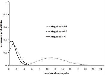
a) Time period 1495-1600

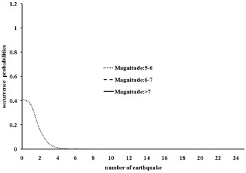
b) Time period 1600-1608

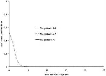
c) Time period 1895-1901

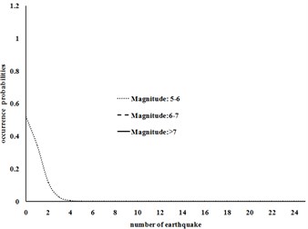
d) Time period 1901-1930

Table 4Probabilities of existence of n missing earthquakes in the time period of 1895-1930 for different magnitude ranges in Tehran

Number of earthquakes ) $n$ (	Time period
	1895-1901			1901-1930
	Magnitude ranges
	5-6	6-7	>7	5-6	6-7	>7
0	5.78E-01	1	1	4.15E-02	1	1
1	3.17E-01	0.0	0.0	1.32E-01	0.0	0.0
2	8.70E-02	0.0	0.0	2.10E-01	0.0	0.0
3	1.59E-02	0.0	0.0	2.23E-01	0.0	0.0
4	2.18E-03	0.0	0.0	1.77E-01	0.0	0.0
5	2.40E-04	0.0	0.0	1.13E-01	0.0	0.0

Fig. 2 shows that for a relatively long period of time interval of 1495-1600, the number of earthquakes with lower magnitude (5-6 with a very high probability of detection probability) follows normal distribution and earthquakes with higher magnitudes (with a relatively low detection probability) have lower bound truncated normal distribution. In the shorter time period (1600-1608) the three curves tend to exponential distribution and reduce the probability of missing earthquakes. The same behavior is observed in the other curves.

It is mandatory to prepare similar tables for each of the consecutive earthquakes in the catalog. Accordingly we generate plausible catalog and now it is possible to produce most probable seismic catalogs based on bootstrap sampling. Table 5 show samples of the completed catalog between 1895 and 1930 A.D. Each row of this table gives the number of earthquake that should be added to the catalog to be completed in the specified time period and magnitude range for given region. Bootstrap duplicates give estimations of $a$ and $b$ values that are used for $a$ and $b$ values mean and standard deviation assessment. Estimated mean and standard deviation of $a$ and $b$ values for Tehran are given in Table 6.

The results are someway different from the previous studies; but they are defendable in terms of the extended study time span (in both ends), historical and recent earthquake addition and inclusion of uncertainty in calculations. Moreover, missing data are regarded in the estimating process. Missing data are usually large earthquakes that can influence seismicity parameters and their variability.

Table 5Probable number of earthquake with different magnitudes in ten bootstrap duplicates for Tehran in 1895-1930 time period

Bootstrsap duplicate	Time period
	1895-1901			1901-1930
	Magnitude ranges
	5-6	6-7	>7	5-6	6-7	>7
1	4	0	0	0	0	0
2	5	0	0	0	0	0
3	10	0	0	2	0	0
4	2	0	0	1	0	0
5	0	0	0	2	0	0
6	12	0	0	5	0	0
7	9	0	0	1	0	0
8	3	0	0	1	0	0
9	2	0	0	1	0	0
10	5	0	0	2	0	0

Considering these data and their uncertainties, can provide more accurate and reliable estimation of seismic hazard. Table 6 shows the effect of the number of bootstrap duplicates on the parameters values. It is obvious from the calculation repetitions (10 times) that a value steady state is attained in 10000 duplicates while its standard deviation converges more rapidly. But in the case of $b$ value the method converge slowly. So, for reliable estimating minimum required duplicate is about 1000000.

Table 6a and b-values based on the proposed method for Tehran

Catalog	$a$	$b$	considerations
Bootstap duplicats of plausible catalog	1.72±0.11	0.83±0.07	$M_{w} \geq$ 5

Table 7a and b-values in bootstrap duplicates

Repetition	Bootstrap duplicates
	1000		10000		100000
	$a$	$b$	$a$	$b$	$a$	$b$
1	1.72±0.11	0.80±0.13	1.72±0.11	1.07±0.10	1.72±0.11	0.90±0.09
2	1.72±0.11	0.69±0.12	1.72±0.11	1.02±0.09	1.72±0.11	0.85±0.08
3	1.71±0.11	0.97±0.17	1.72±0.11	0.67±0.06	1.72±0.11	0.84±0.09
4	1.73±0.11	1.21±0.21	1.72±0.11	0.72±0.06	1.72±0.11	0.82±0.07
5	1.71±0.11	0.71±0.11	1.72±0.11	0.89±0.08	1.72±0.11	0.90±0.07
6	1.72±0.11	0.55±0.09	1.72±0.11	1.01±0.10	1.72±0.11	0.88±0.09
7	1.72±0.11	0.55±0.09	1.72±0.11	1.05±0.09	1.72±0.11	0.82±0.05
8	1.71±0.11	0.65±0.11	1.72±0.11	0.70±0.06	1.72±0.11	0.84±0.05
9	1.71±0.11	1.41±0.25	1.72±0.11	1.08±0.09	1.72±0.11	0.85±0.06
10	1.72±0.11	0.44±0.07	1.72±0.11	0.87±0.07	1.72±0.11	0.83±0.07

5. Conclusion

In this paper, we present a method for improving the accuracy of the PSHA by considering the most plausible seismic data in the maximum possible time period. In order to use the earthquake catalog data in the entire period, we generate plausible catalog based on detection probability. Then, regarding missing earthquakes occurrence probabilities, we offer a probabilistic approach for catalog completing with multiple earthquakes using Bayes’ formula and bootstrap sampling method. So the mean values and standard deviations of G-R law $a$ and $b$ parameters is determined and it is possible to calculate the uncertainty in the PSHA due to these values.

The benefits of this approach can be summarized as follow:

1) The method is practical, especially for parameter $a$ estimation.

2) It takes the advantage of whole catalog utilization probabilistically.

3) It calculates the standard deviation of $a$ and $b$ -values so that we can estimate confidence intervals of PSHA curves.

The performed case study confirms the applicability and efficiency of the proposed method.

References

Šliaupa S. Modelling of the ground motion of the maximum probable earthquake and its impact on buildings, Vilnius city. Journal of vibroengineering, Vol. 15, Issue 2, 2013, p. 532-543.

Search CrossRef
Yan B., Xia Y., Du X. Numerical investigation on seismic performance of base-isolation for rigid frame bridges. Journal of Vibroengineering, Vol. 15, Issue 1, 2013, p. 395-405.

Search CrossRef
Lin W. T., Hsieh M. H., Wu Y. C., Huang C. C. Seismic analysis of the condensate storage tank in a nuclear power plant. Journal of Vibroengineering, Vol. 14, Issue 3, 2012, p. 1021-1030.

Search CrossRef
Gulia L., Meletti C. Testing the b-value variability in Italy and its influence on Italian PSHA. International Journal of Earth scienses, Vol. 49, Issue 1, 2008, p. 59-76.

Search CrossRef
Dong W., Shah H. C., Bao A., Mortgat C. P. Utilization of geophysical information in Bayesian seismic hazard model. International Journal of Soil Dynamics and Earthquake Engineering, Vol. 3, Issue 2, 1984, p. 103-111.

Search CrossRef
Dong W. M., Bao A. B., Shah H. C. Use of maximum entropy principle in earthquake recurrence relationships. Bulletin of the Seismological Society of America, Vol. 74, Issue 2, 1984, p. 725-737.

Search CrossRef
Aki K. Maximum likelihood estimate of b in the formula log N = a – bM and its confidence limits. Bulltein of the Earth Resources Institute, Tokyo University, Vol. 43, 1965, p. 237-239.

Search CrossRef
Kijko A., Sellevoll M. A. Estimation of earthquake hazard parameters for incomplete and uncertain data files. Natural Hazards, Vol. 3, Issue 1, 1990, p. 1-13.

Search CrossRef
Lamarre M., Townsend B., Shah H. C. Application of the bootstrap method to quantify uncertainty in seismic hazard estimates. Bulletin of the Seismological Society of America, Vol. 82, Issue 1, 1992, p. 104-119.

Search CrossRef
Turnbull M. L., Weatherley D. Validation of using Gumbel probability plotting to estimate Gutenberg-Richter seismicity parameters. In Proceedings of the AEES 2006 Conference, Canberra, Australia, 2006.

Search CrossRef
Parsons T. Monte Carlo method for determining earthquake recurrence parameters from short paleoseismic catalogs: example calculations for California. Journal of Geophysical Research, Solid Earth, Vol. 113, Issue B3, 2008, p. B03302.

Search CrossRef
Gutenberg B., Richter C. Seismicity of the earth and associated phenomena. Second edition, Princeton University Press, Princeton, New Jersey, 1954.

Search CrossRef
Utsu T. Aftershocks and earthquake statistics III. Journal of Faculty of Science, Hokkaido, Ser. 7, Geophysics, Vol. 3, 1971, p. 380-441.

Search CrossRef
Kagan Y. Y. Earthquake spatial distribution: the correlation dimension. Geophysical Journal International, Vol. 168, Issue 3, 2007, p. 1175-1194.

Search CrossRef
Gelman A., Meng X. L. Applied Bayesian modeling and Causal inference from incomplete-data perspectives. John Wiley & Sons, London, 2004.

Search CrossRef
Efron B. Bootstrap methods: another look at the jackknife. The Annals of Statistics, Vol. 7, Issue 1, 1979, p. 1-26.

Search CrossRef
Nowroozi A. A., Ahmadi G. Analysis of earthquake risk in Iran based on seismotectonic provinces. Tectonophysics, Vol. 122, Issue 1, 1986, p. 89-114.

Search CrossRef
Niazi M., Bozorgnia Y. The 1990 Manjil, Iran, earthquake: geology and seismology overview, PGA attenuation, and observed damage. Bulletin of the Seismological Society of America, Vol. 82, Issue 2, 1992, p. 774-799.

Search CrossRef
Jafari M. A. The distribution of b-value in different provinces of Iran. The 14th world conference on earthquake engineering, Beijing, China, 2008.

Search CrossRef
Ghodrati A. G., Mahmoudi H., Razavian A. S. Probabilistic seismic hazard assessment of Tehran based on Arias intensity. International Journal of Engineering, Vol. 23, Issue 1, 2010, p. 1-20.

Search CrossRef
Yazdani A., Abdi M. S. Stochastic modeling of earthquake scenarios in greater Tehran. Journal of Earthquake Engineering, Vol. 15, Issue 2, 2011, p. 321-337.

Search CrossRef
Gholipour Y., Bozorgnia Y., Rahnama M., Berberian M., Shojataheri J. Probabilistic seismic hazard analysis, phase I – greater Tehran regions. Final report. Faculty of Engineering, University of Tehran, Tehran, 2008.

Search CrossRef

About this article

Received

12 December 2013

Accepted

14 February 2014

Published

31 March 2014

Keywords

missing earthquakes

seismic catalog homogenization

Gutenberg-Richter law parameters

This is an open access article distributed under the Creative Commons Attribution License, which permits unrestricted use, distribution, and reproduction in any medium, provided the original work is properly cited.