Abstract
Constructing accurate finite element models for engineering structures plays a key role in structural dynamic design and analysis. Finite element model updating using frequency response function data arises great attention. In this paper, a comparison of two model updating approaches by using frequency response function data is investigated. The first method is based on sensitivity analysis, which has been regarded as one of the most successful approaches in model updating. The second one is based on the representation of modeling errors as linear combinations of the individual element matrices, which can be used for both error locating and model updating. The basic formulations of these two methods are introduced and the possible solution strategies are discussed. Numerical simulations are conducted to compare the two model updating methods employing the GARTEUR Truss, two aspects effect on the updating solution including magnitude of initial modeling errors and the completeness of measured coordinates are studied. At last, an experimental cantilever beam is updated by adopting the sensitivity method with tested frequency response function, it is shown that the sensitivity method is effective even when the test data are extremely incomplete.
1. Introduction
Due to the high costs of the experiments, numerical simulations are often adopted to predict the dynamic behavior of engineering structures for reducing the costs in both design and analysis [1, 2]. An accurate numerical model is important in complex structures design, dynamics response computation and safety assessment. Since limited measurement data can be included in the testing model and errors generally exist in the initial finite element model, an accurate numerical model for the purpose of dynamic analysis cannot be obtained by either using test modeling or the finite element modeling. Model updating, a classical inverse problem, is often adopted to reduce the differences between predictions of the finite element model and observations from the dynamics tests, which is an effective way to improve the accuracy of the initial finite element model. It draws great attention from researchers since this technique was proposed, although applying model updating requires a good physical understanding of the structure. Rough finite element models were successfully updated with modal data obtained from experiments in many fields. Recently, Finite element model updating using Frequency Response Functions (FRFs) data draws great attention to researchers owing to several advantages. (1) The FRFs are very sensitive to the damping of structures at resonance peaks, and damping must be included in the finite element model; (2) no modal analysis is required in the updating thus the error in system identification can be avoided; (3) the updating problem is over-determined due to the availability of FRF data at numerous excitation and observation points. All of the above characteristics make the approach with great prospects.
Finite element model updating using frequency response functions has been investigated in recent decades. Surveys on the model updating methods proposed in recent years were discussed by Imregun and Visser [3], and also by Mottershed and Friswell [4]. Definitions on the two different types of error, namely the equation error and the output error, have been proposed by Natke [5] with the weighted least square method to solve the problem in which the damping was not considered. With incomplete measurement data, Foster [6] and Link [7] employed the static and dynamic reduction techniques to condense the system matrix. The truncated modal technique was employed to reduce the system matrix in the state space by Friswell [8]. Imregun and Ewins [9, 10] introduced the basic theory of model updating using frequency response data comprehensively in which the stable solution of the algebraic equations was analyzed without consideration of the measurement noise. A correlation criterion has been explored by Grafe [11] to derivate the formulas of model updating. Attempts had also been made to construct the governing equations for identifying the system matrices with modal expansion and model reduction methods. The modeling and identification of the connections between the two models by using the FRFs data has been investigated by Visser [12].
Amongst the updating methods using FRFs data, the sensitivity method and the system matrix error method are which the researchers pay more attentions to. The former is based on the linearization of a generally non-linear relationship between the selected parameters and the measurement [13]; in the latter method, the errors of the global system matrix are expressed by a linear relation of the element matrix. In this paper, comparison of the two model updating approaches is conducted based on measured data from the GARTEUR Truss. The comparison aims to discuss the application perspectives of the two methods and to provide references for engineers.
2. Basic theory
In this section, basic formulations of the two methods are presented, and then the rules for selecting the frequency points as well as the solution strategies of the updating problem will be briefly introduced.
2.1. The sensitivity method
Starting from the motion equations without considering damping in the frequency domain:
Assuming:
Eq. (1) can be transformed to:
where and are the displacement of the structure and the input force in frequency domain, respectively. is the dynamic stiffness matrix in frequency domain and the inverse of which is the frequency response function , the relationship between and gives:
in which:
The displacement vector can be expressed by:
When a unit force is applied on the th degree-of-freedom (dof) of the structure, on the selected dofs, Eq. (6) can be simplified as:
where is the element at the th row and the th column in the frequency response matrix, the vector denotes the th column of the frequency response matrix.
The error is defined as the difference between the measured and computed response given by:
where is the parameter vector. and is respectively the experimental and the analytical response. Substituting Eq. (6) and (7) into Eq. (8), the residual term gives:
The superscript and denote the FE model and the experimental model respectively. The sensitivity method is developed from a Taylor series expansion in which the high-order terms are truncated, after the truncation, the th column of frequency response function matrix with respect to gives:
where is the sensitivity matrix that can be expressed as:
and are the vector of correction and the number of the parameters need to be updated:
Substituting Eq. (10) into Eq. (9), the residual Eq. (9) can be expressed in the following matrix form:
Assume:
where is the error vector between the experimental and analytical response. After th iterations, if the correlation between the computational and the experimental response is close to 1, the norm of the residual will converged to zero, and the parameter vector is updated to be . Then:
Model updating can be transformed to an iteration problem; the following equations should be solved exactly in every iteration step:
It is noted that the sensitivity matrix is varying during the iteration procedure, and the sensitivity matrix must be calculated at each step until the norm of converged to a small quantity.
The sensitivity method is based on the truncated Taylor expansion, and the solution of Eq. (16) can only identify the error direction of the parameters in a local constraint; however, due to the truncated errors, when the initial parameters contains large errors, the finite element model may not be updated with this method.
2.2. The system matrix error method
Derivation of the system matrix error method begins with the measured frequency response functions, which is briefly introduced in this section.
According to Eq. (1), when a unit force is applied as excitation, the Equations of motion of the experimental model and the analytical model of the system can respectively be written as:
The superscripts and denote FE model and experimental model, respectively.
Assuming that:
where , , are the stiffness, mass and frequency response function errors in the finite element model.
Substituting Eqs. (19) into (18), we have:
Rearranging Eq. (20), it gives:
Substituting Eq. (17) into (21), we have:
Eq. (23) can be employed to solve for the unknown modeling errors. However, before this can be achieved, some parameterization is needed. To parameterize the modeling errors, it is assumed that the error mass and stiffness matrices can be expressed as linear combinations of elemental mass and stiffness matrices, respectively:
where and are the th element mass and stiffness matrices, respectively. and are the perturbation in design parameters corresponding to the element. Notation represents the summation. Substituting Eq. (24) into Eq. (23), we can obtain the following equation:
Eq. (25) can be transformed into a set of linear algebraic equations in terms of unknown perturbations in design parameters which denoted as () and (), respectively:
where , , and are:
Eq. (26) is formulated based on measured response function data with one measurement frequency selected. In practical vibration test, response function data are measured at many different measurement frequencies. When response function data at sufficient number of measurement frequencies are used, Eq. (26) can be transformed as a set of over-determined algebraic equations:
where:
The coefficient matrix and the vector can be calculated in advance which is formed using the analytical model and the measured response function data. Eq. (28) can be solved for using linear least-square method and then the solution is used to reconstruct the updated analytical model together with the original analytical model. However, when the test data is incomplete and contaminated with noise, Eq. (28) is needed to be transformed and constraints have to be added.
2.3. Frequency point selection
Frequency response function are very sensitivity to damping properties at resonance peaks, local modes influence is include and no modal analysis is required, so that it contains much more information than modal data, at each frequency point, the major system information are included. In the updating procedure, because of the huge number of frequency points, it is necessary to select frequency point for improving the convergence speed and the precision, the selected frequencies should ensure the rank of the coefficient matrix in Eqs. (16) or (28) is not less than the number of the parameters which need to be updated, and when the experimental FRF data is contaminated with measurement noises, frequency points selection seems more important.
There are two main principles of frequency are given in references [3, 12]:
1) Choose updating frequencies at the foot of experimental resonances peaks, and
2) Avoid frequencies between corresponding analytical and experimental resonances.
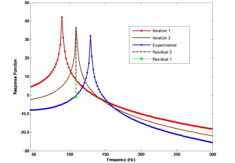
The first rule assures the coefficient matrix in Eqs. (16) or (28) to be well-posed. The second one avoids the problem of large residuals, as shown in Fig. 1, if frequencies between corresponding analytical and experimental resonances are selected, in the process of the analytical data approaching to the experimental frequency response function, the analytical resonances will definitely moving to the select frequency, and the amplitude at resonance is much bigger than the other positions, therefore, the right hand side (Residual 2) may become unbalance easily during the iterations, this will cause the difficulties in solving linear algebraic equations. At each iteration step, it is necessary to ensure the chosen frequencies comply with the rules.
Fig. 1Iteration problem if frequencies are selected between corresponding analytical and experimental resonances
2.4. Solution strategies
Finite element model updating can often be transformed into optimization problem, for accurately reflecting the practical situations and the physical significances of the updated model, and the solution of the optimum solution is often subject to a certain constraint. Due to the above reasons, based on the derivation of the updating theory, the linear algebraic Eq. (16) or (28) can be transformed to an optimization problem with constrains:
where and are respectively the lower limit and the upper limit of the parameter vector . Solving this problem by use of mathematical method to get the estimated vector , the iteration procedure will continue until the norm of converged to a small quantity.
3. Numerical case study
3.1. GARTEUR Truss
The simulation study using a GARTEUR Truss [14] is shown in Fig. 2, which is a cantilever truss. The numerical model of the Truss consists of 78 2-D beam elements, 74 nodes. Each node of the beam element has three dofs (two translations and one rotation) and hence, the total number of dofs in the FE model is 222. The material properties are used in the FE model: Young’s modulus is assumed to be and density . The cross-sectional areas are (horizontal), (vertical), and (diagonal), the bending moment is assumed to be the same for all the elements and is assumed to be .
Fig. 2GARTEUR Truss model
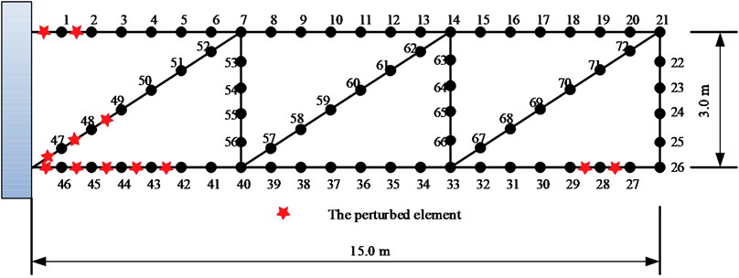
Two simulated cases are carried out based on the GARTEUR Truss model. For Case-I, in order to generate the experimental data, stiffness modeling errors are introduced in the elements of the analytical model of the structure by changing the bending stiffness of elements as shown in Table 1, assuming that the stiffness of element shown in Table 1 are all overrated 20 % in the FE model. While in Case-II, the stiffness of elements in the FE model is overrated or underestimated have apparent discrepancies, details are shown in Table 2.
Table 1Stiffness modeling errors location (case 1)
Element no. | 1 | 2 | 28 | 29 | 43 | 44 | 45 | 46 | 47 | 48 | 49 | 50 |
Error (%) | –20 | –20 | –20 | –20 | –20 | –20 | –20 | –20 | –20 | –20 | –20 | –20 |
Table 2Stiffness modeling errors location (case 2)
Element no. | 1 | 2 | 28 | 29 | 43 | 44 | 45 | 46 | 47 | 48 | 49 | 50 |
Error (%) | –90 | –90 | 100 | 100 | 100 | 100 | 10 | –90 | –90 | –90 | –90 | –90 |
The two cases are employed to investigate the two methods introduced in Section 2, the updated results of coordinates incomplete and coordinates complete are discussed. Considering the small modeling error firstly, and then the large modeling errors.
3.2. Updated results evaluation criterions
To assess the progress of iterations and to compare different updated models certain model quality indices have been constructed. Percentage average error in natural frequencies (AENF) is calculated using following expressions:
where and are the natural frequencies, is the number of the considering modes. The updated model should have the abilities of reflect the test results in the considering frequency domain, outside of which the test results predicted.
Percentage average error in parameters (AEP) is calculated as error in the predicted parameters as a percentage of the known exact parameters:
where is the number of the parameters, and are the value of the parameters.
3.3. Results and discussions
In order to demonstrate their practical application, the two model updating methods using frequency response function of GARTEUR Truss model which is introduced in Section 3.1. For comparative investigation on these methods, two cases including small modeling error and large modeling error are studied. In each case, the measured coordinates complete and incomplete are investigated, the complete case means the response of all coordinates of the structure can be tested, and the incomplete case meaning only translation degree of freedoms can be obtained.
3.3.1. Case-I small modeling error
For the sensitivity method, calculation of the frequency response function matrix with respect to the parameter vector is very time-consuming, and a more important question is that the sensitivity matrix will easily become ill-posed, therefore, the selection of parameters to be updated is also a very important aspect. In this case study, at first, we select the stiffness of all elements in the structure as parameters, the equation is an ill-posed problem, it is hard to get a credible solution. However, assume the position of the errors are known in advance, and select appropriate frequency points, iteration process is required during updating. The identification of element modeling errors is shown in Fig. 3. It can be seen that all the introduced modeling errors are well identified after convergence. The response function curves of the experimental, analytical and updated models are shown in Fig. 4.
Fig. 3Comparison of the exact and identified modeling errors (method 1, coordinates incomplete)

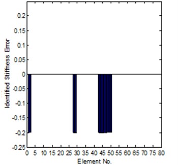
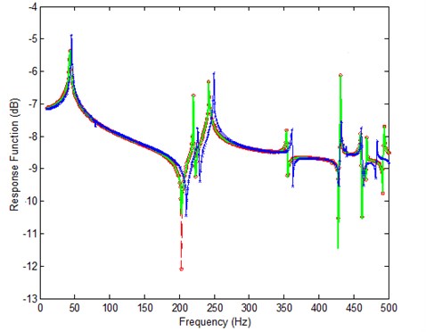
Fig. 4Comparison of the analytical, the experimental and the updated response function curves (method 1) (—o— updated, —— experimental, —*— analytical)
With regard to the second method, for the case of coordinates complete, it is need not to consider many limitations, the frequency point can be selected randomly, the identification of element modeling errors is shown in Fig. 5, and it is found that the agreement between the exact error and the identified error is excellent. But, in vibration test, it is not realistic that all coordinates which are specified in the analytical model have been measured. Therefore, the effect of coordinate incompleteness upon the updating procedure should be assessed. For the case of incomplete data, the model condensation and coordinates expansion technique should be used to solve this problem. In this work, those unmeasured elements of the response function vector are replaced by their analytical counterparts. The results for the identification of element modeling errors are shown in Fig. 6. The response function curves of the experimental, analytical and updated models are shown in Fig. 7. From this figure, there are a few differences between the regenerated and experimental response function data.
Fig. 5Comparison of the exact and identified modeling errors (method-2, coordinates complete)
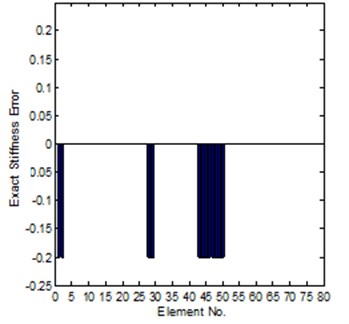
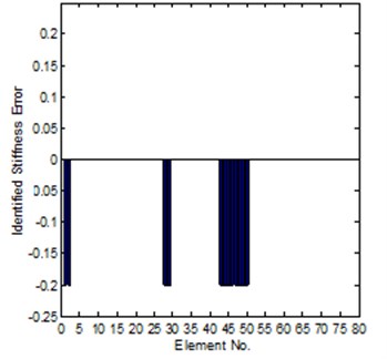
Table 3 is the error indices comparison for the Case-I of small modeling error, from the table it is can be found that, under coordinates complete condition, method-2 can get an excellent solution.
Fig. 6Comparison of the exact and identified modeling errors (method-2, coordinates incomplete)

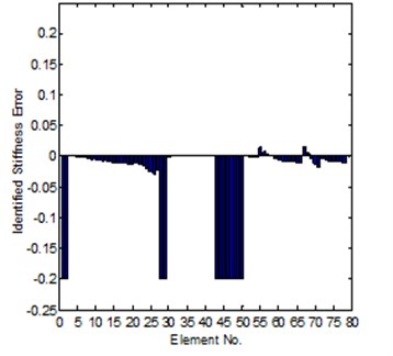
Fig. 7Comparison of the analytical, the experimental and the updated response function curves (method-2) (—o— updated, —— experimental, —*— analytical)
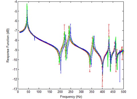
Table 3Error indices comparison for the Case-I of small modeling error (%)
Experimental coordinates | Percentage average error in natural frequencies (AENF) | Percentage average error in parameters (AEP) | ||||
Before updating | Updated | Before updating | Updated | |||
Method-1 | Method-2 | Method-1 | Method-2 | |||
Coordinates complete | 2.82 | – | 0 | 20 | – | 0 |
Coordinates incomplete | 2.82 | 0.01 | 0.18 | 20 | 0.08 | 0.59 |
3.3.2. Case-II large modeling error
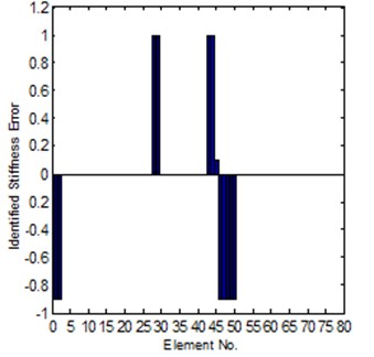
For Case-II, the modeling error is much larger. It is hard to get a convergent solution by using of the sensitivity method; the reason is introduced in Section 2.1. But for the system matrix error method, in the case the coordinates is completely can be tested, it is also easy to get a reliable solution, the results can be seen in Fig. 8 and Fig. 9, it is shown that the solution is close to the exact error. However, for the case of incomplete coordinates, it is not easy get a convergent updating solution. But if we know the stiffness error position in advance, under this condition, the identification of stiffness error can be obtained. The comparison of the exact and identified modeling errors is shown in Fig. 10.
Fig. 8Comparison of the exact and identified modeling errors (method-2, coordinates complete)
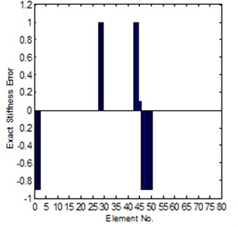
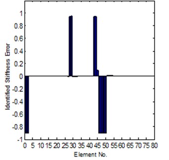
Fig. 9Comparison of the analytical, the experimental and the updated response function curves (method-2) (—o— updated, —— experimental, —*— analytical)
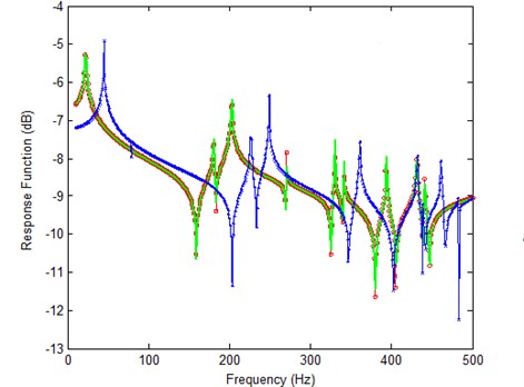
Fig. 10Comparison of the exact and identified modeling errors (method-2, known error position in advance)

4. Experimental case study
A cantilever beam is updated by using the sensitivity method with experimental frequency response function. Geometric dimensions, including cross section and length of the rectangle tube, arrangement of excitation and accelerometer in experimentation are shown in Fig. 11 and Fig. 12. The tube is made of steel, the density and Young’s module of which are respectively and . In this case, the experimental FRF data is obtained by using impact testing with single input single output method; and the measuring direction is along with axis as shown in Fig. 12. The range of sample frequency is 0-2000 Hz.
The cantilever beam is modeled using beam element, three kinds of attributes (-) are assigned to six elements (element ①-⑥) which near the fixed end, is assigned to rest twenty elements of the beam, the full finite element model consist of 27 nodes, 26 beam elements, and 156 active degrees of freedom.
Fig. 11Experimental setup of the impact testing
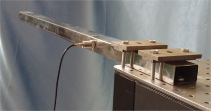
Fig. 12The cantilever beam (Unit: mm)
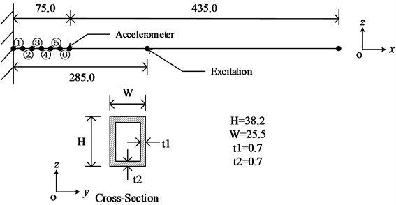
Fig. 13Comparison of the analytical, the experimental and the updated response function curves (—o— updated, —— experimental, —*— analytical)
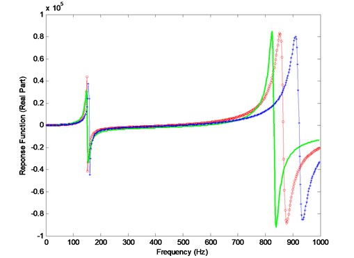
Table 4Variation of parameters after model updating
Parameters | Initial values | Updated | Variation (%) |
(N/m2) | 2.0×10¹¹ | 1.86×10¹¹ | –7.0 |
(N/m2) | 2.0×10¹¹ | 1.73×10¹¹ | –13.5 |
(N/m2) | 2.0×10¹¹ | 1.72×10¹¹ | –14.0 |
(N/m2) | 2.0×10¹¹ | 1.83×10¹¹ | –8.5 |
are selected parameters to be updated in the experimental case study. Comparison of the analytical, experimental, and updated response functions are shown in Fig. 12. The updated parameters are shown in Table 4. It is shown that, after model updating, the finite element model can more accurately reflect the dynamic characteristics in the frequency domain of 0-1000 Hz.
5. Conclusions
Two model updating methods using frequency response function data have been investigated. On the basis of results from the comparative study, the following conclusions are drawn.
1) When the position of modeling errors are known in advance, the sensitivity method is good for solve the case with small errors. And it is difficult to get a convergent solution by using of the sensitivity method when the initial error is large, this indicated that the initial value of parameters to be updated and the optimization constraints are important.
2) With regard to the system matrix error method. Under the condition of coordinates are measured completely, the frequency point can be selected randomly, and it is found that the agreement between the exact error and the identified error is excellent even when large modeling error exists; this method can also be used for localizing the inaccurate parameters. For the case of incomplete coordinates, it is not easy get a convergent updating solution. However, if we know the stiffness error position in advance, the identification of stiffness error can be obtained.
3) The experimental cantilever beam is updated by adopting the sensitivity method with tested frequency response function, it is shown that the sensitivity method is effective even when the test data are extremely incomplete.
References
-
Ma X., Yu D., Han Z., Zou Y. Research evolution on the satellite-rocket mechanical environment analysis and test technology. Journal of Astronautics, Vol. 27, Issue 3, 2006, p. 323-331, (in Chinese).
-
Ding J., Han Z., Ma X. Finite element verification strategy of large complex spacecraft. Journal of Astronautics, Vol. 31, Issue 2, 2010, p. 547-555, (in Chinese).
-
Imregun M., Visser W. J. A review of model updating techniques. The Shock Vibration Digest, Vol. 23, Issue 1, 1991, p. 9-20.
-
Mottershead J. E., Friswell M. I. Model updating in structural dynamics: a survey. Journal of Sound and Vibration, Vol. 167, Issue 2, 1993, p. 347-375.
-
Natke H. G. Updating computational models in the frequency domain based on measured data: a survey. Probabilistic Engineering Mechanics, Vol. 3, Issue 1, 1988, p. 28-35.
-
Foster C. D. A method of improving finite element models by using experimental data: application and implications for vibration monitoring. International Journal of Mechanical Science, Vol. 32, Issue 3, 1990, p. 191-203.
-
Link M. Identification and correction of errors in analytical models using test data: theoretical and practical bounds. Proceedings of the 8th International Modal Analysis conference, Orlando, Kissimmee, 1990, p. 570-578.
-
Friswell M. I. Updating model parameters from frequency domain data via reduced order model. Mechanical Systems and Signal Processing, Vol. 4, Issue 5, 1990, p. 377-391.
-
Imregun M., Visser W. J., Ewins D. J. Finite element model updating using frequency response function data – I: theory and initial investigation. Mechanical Systems and Signal Processing, Vol. 9, Issue 2, 1995, p. 187-202.
-
Imregun M., Sanliturk K. Y., Ewins D. J. Finite element model updating using frequency response function data – II: case study on a medium-size finite element model. Mechanical Systems and Signal Processing, Vol. 9, Issue 2, 1995, p. 203-213.
-
Grafe H. Model updating of large structural dynamics models using measured response functions. Ph.D. Thesis, Imperial College of Since, Technology and Medicine, University of London, UK, 1998.
-
Visser W. J. Updating structural dynamics models using frequency response data. Ph. D. Thesis, Imperial College of Since, Technology and Medicine, University of London, UK, 1992.
-
Mottershead J. E., et al. The sensitivity method in finite element model updating: A tutorial. Mechanical Systems and Signal Processing, Vol. 25, Issue 7, 2011, p. 2275-2296.
-
Lin R. M., Zhu J. Finite element model updating using vibration test data under base excitation. Journal of Sound and Vibration, Vol. 303, 2007, p. 596-613.
-
Lin R. M., Ewins D. J. Analytical model improvement using frequency response functions. Mechanical Systems and Signal Processing, Vol. 8, Issue 4, 1994, p. 437-458.
About this article

The work described in this paper was supported by a Program for New Century Excellent Talents in University a research grant (NCET-11-0086), a research grant by the National Natural Science Foundation of China (10902024), a Doctoral Program of Higher Education of China (20130092120039), and a project funded by the Priority Academic Program Development of Jiangsu Higher Education Institutions (PAPD-1105007001).
