Transverse vibration analysis of an axially moving beam with lumped mass

Liu, Ning; Yang, Guolai; Chen, Bo

Journal of Vibroengineering

Browse Journal

Submit article

Published: 15 November 2014

Check for updates

Transverse vibration analysis of an axially moving beam with lumped mass

Ning Liu¹

Guolai Yang²

Bo Chen³

^{1, 2}School of Mechanical Engineering, Nanjing University of Science and Technology, No. 200 Xiao Ling Wei Street, Nanjing, 210094, China

³School of Energy and Power Engineering, Nanjing University of Science and Technology, No. 200 Xiao Ling Wei Street, Nanjing, 210094, China

Corresponding Author:

Ning Liu

Cite the article Download PDF

Downloads 1237

Abstract

The transverse vibration and stability of an axially moving simply supported beam with lumped mass is invested. A partial-differential equation governing the transverse vibration of the system is derived from Euler-Bernoulli beam model and Newton’s second law. Based on the Galerkin method, the governing equation is truncated to a set of second order time-varying ordinary differential equations. As the gyroscopic item in the motion equations, the complex mode theory is applied to calculate the natural frequencies of the beam with lumped mass. The effects of axially moving speed, position and weight of the lumped mass on the dynamics and instability of the beam are discussed. The results indicate that the natural frequencies decrease as the axially moving speed and weight of the lumped mass increasing. The first natural frequency decreases first, and then increases with the position of the lumped mass between the two supports while the second natural frequency varies more complicatedly. Therefore, the effect of the lumped mass leads to a lower critical speed of the axially moving system. This implies that the lumped mass tends to make the beam more unstable with reduced natural frequencies.

1. Introduction

Axially moving systems are widely used in production and life, such as power transmission band, belt saws, aerial cable tramways, and elevator cables. If the bending stiffness is concern, this kind of systems can be modeled as axially moving beams. Axially moving systems are usually used for transporting goods, artifacts or passengers, which are called attached subsystems and could be simplified into lumped loads model. The effect of the subsystems should be taken into consideration when one analyzes the inherent characteristics of the axially moving systems. The coupling between lumped mass and axially moving beam makes the system dynamics more complicated and leads to time-varying eigenvalues which are difficult to calculate. Besides the gyroscopic term present in the equation of motion of such systems calls for some special techniques of analysis. The literature relating to the two types of beam vibration, i.e. stationary beams carrying various moving concentrated elements and axially moving system, is abundant. However, the combination of the two kinds of problems is seldom involved in previous research.

The problem of dynamic response of beams subjected to moving loads, such as railway bridges or highway bridges under the influence of trains and automobiles, has been studied by many researchers. Inglis [1] made an excellent work on the subject in which many parameters were taken into account. Michaltsos and Sophianopoulos [2], Michaltsos [3] studied the dynamic behavior of a single-span beam subjected to a moving load of constant magnitude and variable velocity. Uzzal and Bhat [4] investigated the dynamic response of an Euler-Bernoulli beam under constant moving load as well as moving mass. The results showed that the moving mass has significantly higher effect on the dynamic responses of beam than the moving load. However, it should be mentioned that the dynamic behaviors of the beam studied above are much different from that of axially moving beam. The deflections of the beam subjected to a moving mass as shown in [3-4] are single peak which are similar to sine curves. However, if the axially moving speed of beam is considered, the dynamic responses show oscillation features. So the natural characteristics and stabilities which are not studied in [3-4] will be discussed in detail in this paper. Mallik and Chandra [5] investigated the steady state response of a beam placed on an elastic foundation and subjected to a concentrated load moving with a constant speed. It was observed that the steady state is not attained at supercritical speed of the load in the ideal undamped case.

The dynamic behavior of axially moving system has been extensively studied since the middle of the 20th century, and is initially focused on the vibration of oil pipelines [6]. An extensive literature overview can be found in reference [7]. For the axially moving system, the dynamic behavior is greatly influenced by axially the moving speed. When a critical value of the axial speed is reached, the first linear natural frequency vanishes; the straight equilibrium position loses stability and bifurcates into new equilibrium states. In the sub-critical speed range, all natural frequencies decrease as the axial speed increases and the vibration modes are complex. Wickert and Mote [8] presented a complex modal method for axially moving continua including beams where natural frequencies and modes associated with free vibration serve as a basis for analysis. Öz and Pakdemirli [9] studied the natural frequency varying with time-dependent velocity for various flexural stiffness values for the first two modes. Principal parametric resonances, sum and difference-type combination resonances are investigated. Öz [10] computed natural frequencies of an axially moving beam in contact with a small stationary mass under pinned-pinned or clamped-clamped boundary conditions. Chen and Yang [11] derived two different models governing transverse motion of a linear elastic moving beam of which geometric nonlinearity was considered to study the nonlinear free vibration. Pellicano and Vestroni [12] established an integro-partial-differential equation governing the transverse motion for an axially moving beam, and used the Galerkin method to discretize the governing equation to study the stability and bifurcation. Ding and Chen [13] calculated the first two natural frequencies of planar vibration of axially moving beams in the supercritical regime by the Galerkin truncation to the coupled longitudinal-transverse governing equations. Depending upon the physical system, either a linear model or a nonlinear model may be considered for the problem. Chakraborty and Mallik [14] derived both the linear and non-linear complex normal modes of a simply supported travelling beam in the light of harmonic wave propagation. It was observed that the effect of the non-linear terms on the beam vibration is weak, and only when the beam travels with a speed close to the critical speed, the effects of nonlinearities have to be considered.

It appears that, to the authors’ knowledge, there have been very few studies on the axially moving beam with lumped mass. The attention of the present investigation is focused on the effect of lumped mass on the behavior of the beam. This paper is organized as follows. It first derives the governing equation of motion for transverse vibrations of an axially moving simply supported beam with lumped mass. Then the Galerkin method is proposed to discretize the equation of motion as well as the boundary conditions. After that the natural frequencies and modes are investigated with the complex mode approach. Finally the effects of lumped mass on vibration characteristics and critical speed are analyzed.

2. Governing equation of motion

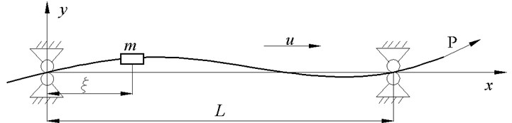
Consider a tensioned beam, with lumped mass $m$ , density $ρ$ , cross-sectional area $A$ , area moment of inertia of the cross-section about neutral axis $I$ , modulus of elasticity $E$ , axially tension $P$ , traveling at a constant axial speed v between two simple supports separated by distance $L$ , as shown in Fig. 1. Introduce a fixed Cartesian coordinate system $x y z$ taking one end of the beam as the origin. Out-of-plane motion and vibration of the cross-sectional dimensions are not taken into account. The beam is modeled based on the Bernoulli-Euler beam theory where shear deformation is neglected. The Newton second law of motion yields:

1

ρ A (y_{, t t} + 2 u y_{, x t} + u^{2} y_{, x x}) - P y_{, x x} + E I y_{, x x x x}

= - m (g + y_{, t t} + 2 u y_{, x t} + u^{2} y_{, x x}) \cdot δ (x - s),

where a comma preceding $x$ or $t$ denotes partial differentiation with respect to $x$ or $t$ , $δ$ is the Dirac delta function.

Fig. 1Schematic of simply supported axially moving beam with lumped mass

In the present investigation, the boundary conditions of the beam which is simply supported at both ends are considered as follows:

2

y (0, t) = y (L, t) = 0, y_{, x x} (0, t) = y_{, x x} (L, t) = 0 .

Introduce the dimensionless variables and parameters as follow:

3

w = \frac{y}{L}, ξ = \frac{x}{L}, τ = t \sqrt{\frac{P}{ρ A L^{2}}}, c = u \sqrt{\frac{ρ A}{P}},

v_{f}^{2} = \frac{E I}{P L^{2}}, α = \frac{m}{ρ A L}, γ = \frac{s}{L}, β = \frac{ρ A L g}{P} .

Eq. (1)-(2) can be respectively cast into the dimensionless form:

4

w_{, τ τ} + 2 c w_{, ξ τ} + (c^{2} - 1) w_{, ξ ξ} + v_{f}^{2} w_{, ξ ξ ξ ξ} = - α (β + w_{, τ τ} + 2 c w_{, ξ τ} + c^{2} w_{, ξ ξ}) \cdot δ (ξ - γ),

5

w (0, τ) = w (1, τ) = 0, w_{, ξ ξ} (0, τ) = w_{, ξ ξ} (1, τ) = 0 .

3. Discretization of the equation of motion

In general, analytical solutions for the governing Eq. (4) are difficult to find. The Galerkin method is widely used for the spatial discretization of an axially moving continuum. In this paper, the Galerkin method is employed to analyze the beam problem. The displacement field $w (ξ, τ)$ is expanded in a series of suitable trail functions $ϕ_{i} (ξ)$ and truncating the series at the $N$ th term. The basis $ϕ_{i} (ξ)$ must be a complete and linearly independent set of functions and respect for the boundary conditions. Usually the eigenfunctions are good choice. In the present study, the eigenfunctions of a stationary beam with simply supports are chosen as the trail functions, i.e. the sine series, which also fits the present problem:

6

w (ξ, τ) = \sum_{i = 1}^{N} ϕ_{i} (ξ) η_{i} (τ),

7

ϕ_{i} (ξ) = s i n (i π ξ), i = 1,2, \dots, N,

where $η_{i} (τ)$ is defined as the generalized coordinates. The number $N$ depends on the convergence of the sine series, and is linked to the smoothness of the function $w (ξ, τ)$ . Eq. (6) could be written in matrix-vector form as:

8

w (ξ, τ) = ϕ^{T} (ξ) \cdot η (τ) .

Substituting Eq. (8) into Eq. (4), multiplying Eq. (4) by $φ (ξ)$ , and then integrating the equation from $ξ =$ 0 to 1, we obtain the following set of second-order ordinary differential equations:

9

M \ddot{η} (τ) + C \dot{η} (τ) + K η (τ) = F (τ),

where a superscript dot represent derivative with respect to time, $M$ , $C$ and $K$ are structural mass matrix, damping matrix and stiffness matrix, respectively. The formulation of these coefficient matrixes are given by:

10

M = \int_{0}^{1} φ φ^{T} d ξ + α φ (γ) φ^{T} (γ),

11

C = 2 \int_{0}^{1} c φ {φ^{'}}^{T} d ξ + 2 α c φ (γ) {φ^{'}}^{T} (γ),

12

K = \int_{0}^{1} (c^{2} - 1) φ {φ^{″}}^{T} d ξ + \int_{0}^{1} v_{f}^{2} φ^{″} {φ^{″}}^{T} d ξ + α c^{2} φ (γ) {φ^{″}}^{T} (γ),

13

F = - α β φ (γ) .

4. Complex mode analysis

For travelling beams the eigenfunctions are complex and dependent on the axially speed due to the gyroscopic item in the discretized motion Eq. (9). Thus, the complex mode theory is applied to calculate the natural frequencies of the system. Introduce the state space vector:

14

q = (\begin{matrix} \dot{η} \\ η \end{matrix}) .

Eq. (9) is represented in the state space as follows:

15

\tilde{M} \dot{q} + \tilde{K} q = f,

where:

16

\tilde{M} = (\begin{matrix} 0 & M \\ M & C \end{matrix}), \tilde{K} = (\begin{matrix} - M & 0 \\ 0 & K \end{matrix}), f = (\begin{matrix} 0 \\ F \end{matrix}) .

The homogeneous equation associated with Eq. (15) which corresponds to a generalized eigenvalue problem is given by:

17

\tilde{M} \dot{q} + \tilde{K} q = 0 .

The solution of Eq. (17) can be written in the following form:

18

q = ψ e^{λ t},

where $ψ$ is the eigenvector, $λ$ is an eigenvalue. Substituting Eq. (18) into Eq. (17) leads to the eigenvalue problem:

19

(λ \tilde{M} + \tilde{K}) ψ = 0 .

To obtain a non-trivial solution of the above equation, it is required that the determinant of the coefficient matrix vanishes, namely:

20

d e t (λ \tilde{M} + \tilde{K}) = 0 .

We can get the complex eigenvalue $λ$ numerically from Eq. (20) which appears in the form of conjugate complex. The positive imaginary part of the eigenvalue denotes the natural frequencies of the axially moving system while the real part indicates the stability of the system. Besides, in order to determine the eigenfunctions $Γ_{i} (x)$ of the axially moving system, the eigenvector $Ψ = [ψ_{1}, ψ_{2}, ψ_{3}, \dots, ψ_{2 N}]$ from Eq. (19) is used for approximated computing:

21

Γ_{n} (x) = \sum_{i = 1}^{N} ϕ_{i} Ψ_{i + N, n},

where $Ψ_{i + N, n}$ indicates the ( $i + N$ , $n$ ) element of the eigenvector matrix $Ψ$ .

5. Numerical results and discussions

5.1. Comparisons with available results

Numerical studies have been conducted to investigate the effects of several key parameters on the vibration characteristics of the axially moving beam with lumped mass.

Fig. 2The lowest two eigenvalues of a simply-supported moving beam vs. axially moving speed with flexural rigidity vf= 1: a) the imaginary part and b) the real part

The lowest two eigenvalues of a simply-supported moving beam vs. axially moving speed with flexural rigidity vf= 1: a) the imaginary part and b) the real part

a)

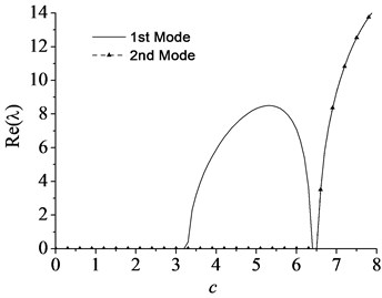
b)

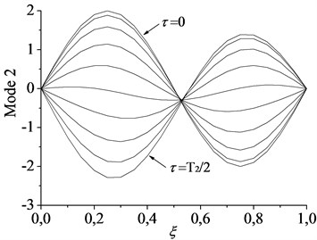
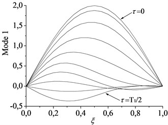
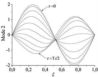
To validate the accuracy of the numerical results and provide comparison for the vibration character of the axially moving beam-mass system, the dynamics of axially moving beam without lumped mass was studied first. The effects of moving speed on the variation of the lowest two eigenvalues of the moving beam with simple supports are given in Fig. 2. The results demonstrate good agreement with reference [9]. It can be observed that the imaginary parts of eigenvalues (i.e., natural frequencies) decrease as the moving speed is increased up to the lowest critical speed $c_{c r} =$ 3.3. Here, the lowest critical speed is defined as when the speed exceeds the definite value, the imaginary part of eigenvalue $λ_{1}$ (i.e., the first natural frequency) vanishes completely while its real part turns to positive from zero. This implies that the main diagonal element $K_{11}$ of the stiffness matrix in Eq. (9) comes into negative and the first natural frequency becomes unstable by the divergence instability when the moving speed becomes equal or larger than the lowest critical speed of about 3.3. The complex nature of the eigenfunction $Ψ_{i}$ leads to the nonstationary, linear normal mode-shapes which change during the period in a single mode vibration. This phenomenon can be illustrated in Fig. 3 where a dynamic representation of the first two modes is shown when $c = 1$ . In this case, a linear mode shape is given as initial condition, i.e. $w (ξ, 0) = s i n (π ξ)$ and $w (ξ, 0) = s i n (2 π ξ)$ for the first two modes vibration, respectively. In order to make the vibration process clear, the shapes of motion are depicted within half a period (i.e. $T_{1} = 2 π / I m (λ_{1})$ , $T_{2} = 2 π / I m (λ_{2})$ when $c = 1$ ). It should be noticed that, although the curves seem to go through the same point in the second mode vibration, there are no nodal positions preserved during the vibration process, which could be observed more obviously when the bending stiffness $v_{f}$ decreases enough (see reference [12]).

Fig. 3Spatial forms of the first two modes in half a period of oscillation for c= 1: a) first mode and b) second mode

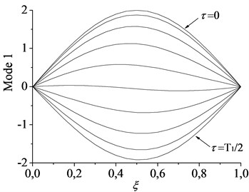
a)

b)

5.2. Effect of moving speed on the stability of the axially moving beam-mass system

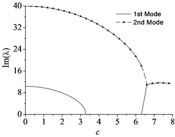
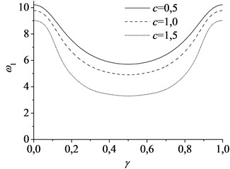
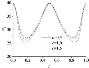
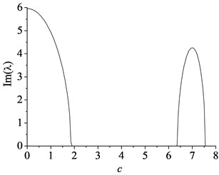
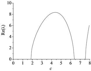
The eigenvalues of the axially moving beam-mass system rely on the position of the mass between two supports when the synchronously moving lumped mass is taken into account. In fact, the axially moving beam with lumped mass is a time-varying system and possesses the inherent characteristics quite different from the axially moving beam. Using the dimensionless parameters $α =$ 1, $v_{f} =$ 1, the natural frequencies with the position of the mass between two supports are given in Fig. 4 for the first and second modes, respectively, for different axially moving speed. The numerical simulations indicate that the first natural frequency decreases first, and then increases with the displacement of the lumped mass. The frequency get the minimum value when the mass is located at the midpoint of the beam. The second natural frequency with the displacement of the lumped mass is quite different from that of the first mode and resembles the shape of “W”. Besides, there is a similar regular pattern that frequencies of beam-mass system also decrease with the increasing speed. Therefore, the first natural frequency takes the lead in decreasing to zero with the increasing axially moving speed when the mass is located at the midpoint of the beam (see Fig. 4). Fig. 5 shows the lowest critical speed $c_{c r} =$ 1.9 of the beam-mass system which implies that the first natural frequency becomes unstable by the divergence instability. However, the critical speed of the beam-mass system is much smaller than that of pure axially moving beam shown in Fig. 2. For 1.9 $< c <$ 6.3, the first natural frequency keeps divergence instability. For 6.3 $< c <$ 7.6, the imaginary part of $λ_{1}$ increases first, and then decreases with the increasing speed while the real part of $λ_{1}$ gets to zero again. This implies that the first natural mode will become stable during the speed range. If $c >$ 7.6, the imaginary part of $λ_{1}$ becomes zero while the real part of $λ_{1}$ keeps positive. Similarly as before, this means that the first natural frequency will become divergence instability. Fig. 6 shows the spatial forms of first two modes vibration process of the beam-mass system in half a period for $c =$ 1, $α =$ 1. It can be seen that the effect of moving mass on the response of the first mode vibration is more notable than the others.

Fig. 4The natural frequencies varying with the movement of the mass at different axially speed: a) the first mode and b) the second mode, using parameter α= 1, vf= 1

The natural frequencies varying with the movement of the mass at different axially speed: a) the first mode and b) the second mode, using parameter α= 1, vf= 1

a)

b)

Fig. 5The minimum value of the first natural frequency with the axially moving speed: a) the imaginary part and b) the real part

a)

b)

Fig. 6Spatial forms of the first two modes of beam-mass system in half a period of oscillation for c= 1, α= 1: a) first mode and b) second mode

a)

b)

5.3. Effect of lumped mass weight on the stability of the axially moving beam-mass system

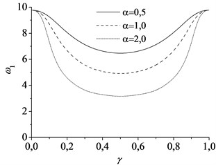
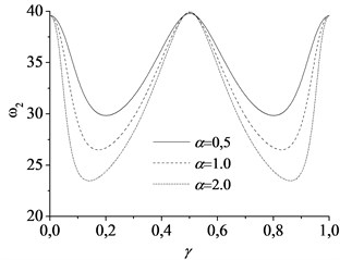
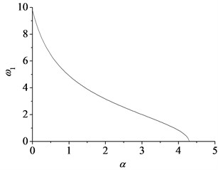
Fig. 7 shows the effects of the mass weight on the natural frequencies for first and second modes of the axially moving beam with the parameters. In present calculation, $c =$ 1, $v_{f} =$ 1. In Fig. 7, the three types of line stand for the natural frequencies at three different dimensionless mass weight $α =$ 0.5, 1.0 and 2.0, respectively. The comparisons indicate that the natural frequencies decrease with the growth of the mass weight. In order to investigate the effects of the lumped mass on the critical speed, Fig. 8 shows the minimum value of the first natural frequency varying with the mass weight. When the mass weight $α =$ 4.3, the first natural frequency decreases to 0 and the system will become instability. Comparing with the critical speed mentioned above, here, the mass could be defined as critical mass. Therefore, the stability of axially moving beam-mass system depends on not only the axially moving speed, but also the mass weight.

Fig. 7The natural frequencies varying with the movement of the mass at different magnitude of mass: a) the first mode and b) the second mode, using parameter c= 1, vf= 1

The natural frequencies varying with the movement of the mass at different magnitude of mass: a) the first mode and b) the second mode, using parameter c= 1, vf= 1

a)

b)

Fig. 8The minimum value of the first natural frequency with the mass weight

6. Conclusions

In this paper, the vibration characteristics of an axially moving beam with lumped mass is investigated. Since the gyroscopic term in the motion equation, the mode shape of a travelling beam is not stationary in space. The complex mode analysis is used to obtain the non-stationary complex normal modes. The results show that the first natural frequency decreases first, and then increases with the displacement of the lumped mass and the frequency get the minimum value when the mass is located at the midpoint of the beam. The natural frequencies of the beam-mass system decrease with the increasing of the axially moving speed and mass weight. When the parameters get to the critical speed or critical mass, the first natural frequency decreases to zero and the system becomes instability. Therefore, it is necessary to pay attention to the effect of axially moving speed and weight of lumped mass simultaneously on the stability of axially moving beam-mass system in engineering.

References

Inglis S. C. E. A Mathematical Treatise on Vibrations in Railway Bridges. Cambridge University Press, Cambridge, 1934.

Search CrossRef
Michaltsos G., Sophianopoulos D., Kounadis A. N. The effect of a moving mass and other parameters on the dynamic response of a simply supported beam. Journal of Sound and Vibration, Vol. 191, Issue 3, 1996, p. 357-362.

Search CrossRef
Michaltsos G. T. Dynamic behaviour of a single-span beam subjected to loads moving with variable speeds. Journal of Sound and Vibration, Vol. 258, Issue 2, 2002, p. 359-372.

Search CrossRef
Uzzal R. U. A., Bhat R. B., Ahmed W. Dynamic response of a beam subjected to moving load and moving mass supported by pasternak foundation. Shock and Vibration, Vol. 19, Issue 2, 2012, p. 201-216.

Search CrossRef
Mallik A. K., Chandra S., Singh A. B. Steady-state response of an elastically supported infinite beam to a moving load. Journal of Sound and Vibration, Vol. 291, Issue 3, 2006, p. 1148-1169.

Search CrossRef
Ashley H., Haviland G. Bending vibrations of a pipe line containing flowing fluid. Journal of Applied Mechanics, Vol. 17, Issue 3, 1950, p. 229-232.

Search CrossRef
Wicker J., Mote Jr. C. Current research on the vibration and stability of axially-moving materials. The Shock and Vibration Digest, Vol. 20, Issue 5, 1988, p. 3-13.

Search CrossRef
Wickert J., Mote C. Classical vibration analysis of axially moving continua. Journal of Applied Mechanics, Vol. 57, Issue 3, 1990, p. 738-744.

Search CrossRef
Öz H., Pakdemirli M. Vibrations of an axially moving beam with time-dependent velocity. Journal of Sound and Vibration, Vol. 227, Issue 2, 1999, p. 239-257.

Search CrossRef
Öz H. Natural frequencies of axially travelling tensioned beams in contact with a stationary mass. Journal of Sound and Vibration, Vol. 259, Issue 2, 2003, p. 445-456.

Search CrossRef
Chen L. Q., Yang X. D. Nonlinear free transverse vibration of an axially moving beam: comparison of two models. Journal of Sound and Vibration, Vol. 299, Issue 1, 2007, p. 348-354.

Search CrossRef
Pellicano F., Vestroni F. Nonlinear dynamics and bifurcations of an axially moving beam. Journal of Vibration and Acoustics, Vol. 122, 2000, p. 21-30.

Search CrossRef
Ding H., Chen L. Q. Galerkin methods for natural frequencies of high-speed axially moving beams. Journal of Sound and Vibration, Vol. 329, Issue 17, 2010, p. 3484-3494.

Search CrossRef
Chakraborty G., Mallik A. K. Wave propagation in and vibration of a travelling beam with and without non-linear effects, part I: Free vibration. Journal of Sound and Vibration, Vol. 236, Issue 2, 2000, p. 277-290.

Search CrossRef

About this article

Received

26 January 2014

Accepted

07 April 2014

Published

15 November 2014

Keywords

axially moving beam

lumped mass

natural frequency

transverse vibration

Acknowledgements

This work is supported by the National Basic Research Program of China (973 Program) (No. 61311603).

This is an open access article distributed under the Creative Commons Attribution License, which permits unrestricted use, distribution, and reproduction in any medium, provided the original work is properly cited.