Abstract
Dynamic behaviour of a semi-infinite elastic beam subjected to a moving single sinusoidal pulse was investigated by using finite element method associated with dimensionless analysis. The typical features of the equivalent stress and beam deflection were presented. It is found that the average value of maximal equivalent stress in the beam reaches its maximum value when the velocity of moving pulse is closed to a critical velocity. The critical velocity decreases as the pulse duration increases. The material, structural and load parameters influencing the critical velocity were analysed. An empirical formula of the critical velocity with respect to the speed of elastic wave, the gyration radius of the cross-section and the pulse duration was obtained.
1. Introduction
With the development of high-speed trains, dynamic behaviour of trains subjected to aerodynamic force attracts increasing research interests. Some aerodynamic problems, such as air pressure pulse occurring as two trains pass each other, aerodynamic drag and pressure waves inside tunnel, are usually neglected in the design of low-speed trains, but they should be considered in the design of high-speed trains [1]. The air pressure pulse may cause the instability of carriage structures [2]. To guide carriage structure design, it is necessary to understand the mechanism of interaction between moving pulse and stress wave in structures.
The air pressure pulse that occurs as two trains pass each other and acts on the trains was investigated by some researchers [1]. A sample of the air pressure pulses measured in the middle carriage of train is shown in Fig. 1 [3]. The typical feature of the pressure fluctuation is of alternating positive and negative values. The positive-negative pressure fluctuation is caused by the fore-body of a train passing the other train, while the negative-positive pressure fluctuation is caused by the after-body of a train passing the other train. These air pressure pulses travel along the side of trains. Raghunathan et al. [1] found that the time interval between the positive and the negative peak pressure values is inverse-proportional to the relative speed of trains. This means that the spatial interval between the positive- and the negative-peak pressure values is constant. They also found that the peak value of air pressure pulse is proportional to the square of the relative speed of trains. As the new generation trains speed up, the peak value of air pressure pulse will become very large, which may seriously endanger the safety of trains.
The moving load problems may be met in many fields of transportation, such as tunnel, rail and launcher. One of the moving load problems was firstly raised from trains passing through railway bridges [4]. Three main kinds of moving load, i.e. moving concentrated force [5-7], partially distributed moving mass or forces [8, 9], and successive point load [10, 11], have been studied. An interesting phenomenon is that the moving load which travels at a certain velocity will cause significant vibration of a structure. For the case of a single moving constant force, Timoshenko [5] found that there exists a critical velocity when applied the force to a finite spatial length Euler-Bernoulli beam resting on an elastic Winkler foundation. The critical velocity is dependent on the stiffness parameter of the elastic foundation, mass of unit spatial length of the beam and the bending stiffness of the cross-sectional area of the beam. For the same kind of load, the critical velocity was found to be equal to the shear wave speed when the structure is a semi-infinite Timoshenko beam without a supporting foundation [6]. When the moving force is harmonic, it should be noted that there is a critical frequency (resonant frequency) which depends on the stiffness parameter of the elastic foundation and mass of unit spatial length of the beam, and the critical velocity is the same as the one in Ref. [5] for an infinite Timoshenko beam on viscoelastic foundation [7]. For the case of partially distributed moving mass or forces, Sun [8] also found a critical velocity for beam-type structures on an elastic foundation. It can be seen that the critical velocity is the same as the first case of moving load for the identical model. The critical velocity was also found in the Bernoulli-Euler model of a beam resting on an elastic foundation [9]. For the case of successive point load, Adams [11] found that the critical velocity is influenced by the value of the load-spacing and much lower than the case of single moving load for a tensioned beam on a damped elastic foundation. All above critical velocities only depend on the geometric and material parameters of beam and the stiffness of the support if used.
Fig. 1Pressure fluctuation caused by trains passing each other [3]
![Pressure fluctuation caused by trains passing each other [3]](https://static-01.extrica.com/articles/14994/14994-img1.jpg)
a)
![Pressure fluctuation caused by trains passing each other [3]](https://static-01.extrica.com/articles/14994/14994-img2.jpg)
b)
However, the features of air pressure pulse considered in this study are very different from the above moving loads. One distinctive feature is that the air pressure pulse has alternating positive/negative amplitude values, as shown in Fig. 1. Another feature is that there is a single period in its load distribution. The dynamic response and its mechanism of a structure subjected to such kind of the air pressure pulse have not been explored.
To understand the dynamic response of an elastic beam to a moving pulse, a finite element model is developed in Section 2. In Section 3, the influence of pulse duration on the critical velocity is studied, several new phenomena are found and the factors influencing the critical velocity are studied by using dimensional analysis. Conclusions are drawn in Section 4.
2. Finite element model
The dynamic response of a beam to a moving pulse is investigated by using finite element method with ABAQUS/Explicit code. According to the knowledge of Fourier analysis, the air pressure pulse can be represented or approximated by sums of trigonometric functions and the main effect comes from the basic frequency. For simplicity, a moving single sinusoidal pulse is used in this study to approximate the air pressure pulse. The beam is considered to be long enough to approximate a semi-infinite beam. Its spatial length is set to be 2000 m and the far end is clamped. A single-period sinusoidal pulse travels from the symmetry boundary to the clamped end of the beam, as schematically represented in Fig. 2. The pulse duration, , ranges from 0.05 to 0.25 s and the pulse amplitude, , is set to be 3 kPa for most cases. The velocity of moving pulse, , is 130-350 m/s. The spatial interval between the positive and the negative peak of the moving pulse, , is 3.25-43.75 m. The cross section of the beam is square with the side length of 0.6 m. The beam is elastic. Its density , Young’s modulus and Poisson’s ratio are 2700 kg/m3, 70 GPa and 0.3, respectively. Timoshenko beam element B32 (quadratic) is selected. According to a convergence analysis, the element length is set to be 0.1 m. The displacement of nodes and equivalent stress of beam elements are recorded. In this study, the equivalent stress is calculated from the von Mises stress of beam element and is denoted as . The maximal equivalent stress of each element, denoted as , and the beam deflection, , are analyzed. To ignore the influence of the reflected wave, the calculation is ceased when the moving pulse moves to position 450 m away from the symmetry boundary, which is larger than 10. Only the equivalent stresses and the beam deflections within the first 300 m are considered.
Fig. 2A single sinusoidal pulse moving along a beam
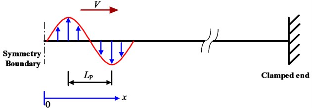
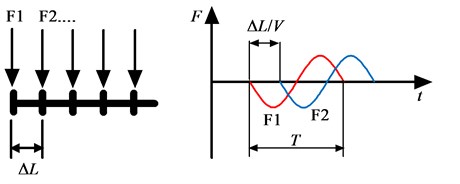
The amplitude of the moving pulse has been simplified to be identical for all cases except for the dimensionless analysis of critical velocity in Section 3.4. Since the beam is elastic, the finite element model is linear. In the finite element model, the pressure applied on the beam is replaced by a set of discrete concentrate forces on relevant nodes. The area between two adjacent nodes is 0.06 m2 and the amplitude of the pulse is 3 kPa, so the peak concentrate force is 180 N, and the temporal interval for the discrete concentrate force set moving one element ahead is , as illustrated in Fig. 3.
Fig. 3The discrete forces on the nodes
3. Results and discussion
3.1. Features of beam deflection
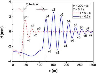
As an example, Fig. 4(a) shows the deflection profiles of beam at two different times, where the velocity of moving pulse and the pulse duration are taken as 200 m/s and 0.1 s, respectively. It is found that the vibration of beam is significant in a particular region in front of the moving pulse. The vibration behind the moving pulse is not significant and the beam deflection is around 3 mm. At time 0.2 s, the amplitude of vibration is small and decays as the distance from the pulse front increases. At time 0.6 s, the vibration in a particular region in front of the moving pulse is relatively stable. With the increase of time, this stable region increases gradually.
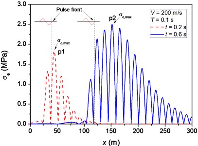
Fig. 4a) Beam deflection and b) equivalent stress vs. position at different times. The symbols “pn” and “vn” denote the nth peak and the nth valley of beam deflection, respectively, ahead of the pulse front
a)
b)
Fig. 5a) Vibration of the node at position 300 m and b) amplitude of deflection vs. frequency of vibration of the node
a)
b)
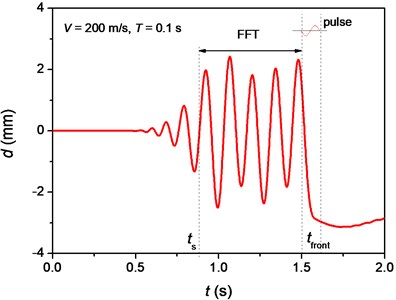
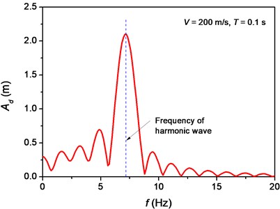
With the transverse vibration of beam, flexural waves propagate along the beam. The wavelength of the flexural waves ahead of the pulse front is approximately equal to the spatial length of the pulse. The phase velocity of flexural wave depends on the main frequency of the flexural wave [12]. As an example, the vibration of the node at position 300 m away from the symmetry boundary was analyzed in Fig. 5. The node is still at first, and then it begins to vibrate when the flexural wave arrives, as shown in Fig. 5(a). After a particular time, denoted as , the node vibrates in a relative stable manner until the moving pulse arrives. In this case, the time when the moving pulse reaches this node, , is 1.5 s. We determined the main frequency of vibration between and with the method of Fast Fourier Transform (FFT). The resulted amplitude of deflection, , vs. frequency of vibration, , curve of the node is shown in Fig. 5(b), where the main frequency is 7.2 Hz. This frequency is in agree with the frequency of harmonic wave travelling at the same velocity as that of moving pulse in an elastic beam, determined by [12]:
where is defined as:
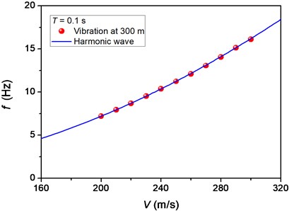
with and being the area and the moment of inertia of the cross-section, respectively. This implies that the phase velocity of flexural wave is equal to the velocity of moving pulse. As shown in Fig. 6, the main frequency of vibration at 300 m is coincided well with the frequency of harmonic wave travelling at the velocity of moving pulse for any velocity of moving pulse. For a particular elastic beam, the main frequency of the flexural wave is not influenced by the spatial length of the moving pulse and only dependent on the velocity of moving pulse.
Fig. 6Comparison between the main frequency of vibration at 300 m and the frequency of harmonic wave for different velocities of moving pulse
3.2. Features of maximal equivalent stress
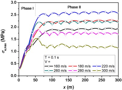
We first take the pulse duration to be 0.1 s but vary the velocity of moving pulse to figure out some features of the distribution of maximal equivalent stress. For a particular velocity of moving pulse, there is two phases for the distribution of maximal equivalent stress. In phase I, the maximal equivalent stress increases as the distance to the symmetry boundary increases until it reaches a maximum value, see Fig. 7(a). In phase II, the maximal equivalent stress is much stable. From Fig. 7(a), it is found that the maximal equivalent stress is influenced by the velocity of moving pulse dramatically.
Fig. 7a) Maximal equivalent stress vs. position and b) the average value of maximal equivalent stress vs. the velocity of moving pulse
a)
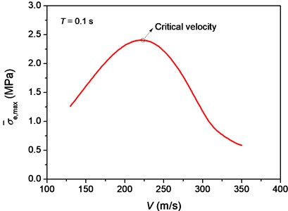
b)
To evaluate the level of maximal equivalent stress in phase II, we evaluate the average value of maximal equivalent stress in this phase, denoted as . The beginning position of phase II is determined by minimizing the variance of . The average beginning position of phase II for the velocities of moving pulse considered in Fig. 7(a) is about 50 m. As the velocity of moving pulse increases, increases first before reaching its maximum value and then decreases, as shown in Fig. 7(b). It is found that achieves its maximum value at a certain velocity, which is termed as the critical velocity. In this case of 0.1 s, the critical velocity is 221 m/s.
The critical velocity is dependent on the pulse duration. We calculated a series of with varying pulse duration and velocity of moving pulse, and the results are shown in Fig. 8. It is found that the critical velocity decreases with increasing pulse duration, but along the line of critical velocity increases with increasing pulse duration.
Fig. 8The variation of σ-e,max with the velocity of moving pulse and the pulse duration: a) three-dimensional diagram and b) a contour plot
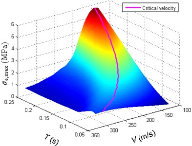
a)
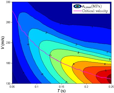
b)
3.3. Mechanism of stress fluctuation
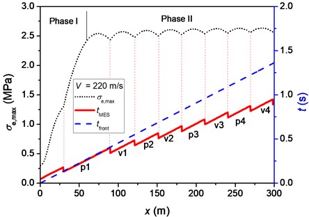
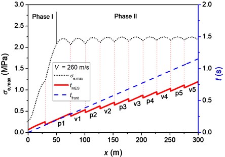
To explore the mechanism of maximal equivalent stress fluctuation with position, we also take the pulse duration of 0.1 s as an example. The variation of with position at phase II is shown in Fig. 9(a).
For each position, the time when is reached, , and the time when the pulse front arrives, , were analyzed. Three velocities of moving pulse, namely 180, 220 and 260 m/s, are considered, which correspond to velocities lower than, closing to and higher than the critical velocity, respectively. The value of means the maximum value of equivalent stress that a specific position ever had. In this beam model, the maximal equivalent stress implies the maximum degree of bending which appears at the peak/valley of the beam deflection. The serial numbers of peaks and valleys are defined in Fig. 4(a). The symbols “p” and “v” denote the th peak and the th valley of beam deflection, respectively, ahead of the pulse front. Fig. 4(b) shows the equivalent stresses in the beam. According to the positions of shown in Fig. 4(b) and the deflection profile of beam shown in Fig. 4, we can determine that appears in p1 and p2 when 0.2 s and 0.6 s, respectively. In this way, the time that appears in peaks and valleys of beam deflection can be determined, as presented in Fig. 9.
It is interesting to find that the position of maximum degree of bending successively appears at p1, v1, p2, and so on, of the beam deflection. The duration of appearing at p1 is longer than those at v1, p2, and so on. This is because that the bending degrees of the following p or v also increase before the position corresponding to p1 attains its maximal bending degree. In phase II, it is found that the positions where attains minimum point are coincident with the positions where the corresponding beam deflection switches from the peak to the valley or vice versa. The travelling speeds of peaks or valleys are the reciprocal of the line slopes of for each corresponding segment. It can be seen from Fig. 9 that the slopes of all parts of the curve are equal to the slope of the time when pulse front arrives versus position curve. Therefore, the travelling speed of p or v is equal to the velocity of moving pulse. This result agrees well with the analysis of main frequency of flexural wave in Section 3.1.
Fig. 9Maximal equivalent stress, σe,max, the time when σe,max is reached, tMES, and the time when the front of moving pulse arrives, tfront, at each position for different velocities of moving pulse: a) 180 m/s, b) 220 m/s and c) 260 m/s. The symbols “pn” and “vn” represent the nth peak and nth valley of beam deflection, respectively, when σe,max is reached
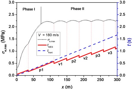
a)
b)
c)
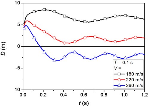
The relative distance between the pulse front and p1, , are pulse-velocity dependent. The variations of for the three typical velocities of moving pulse are shown in Fig. 10. At the beginning time, they are almost identical but then fluctuate around different levels. It can be seen that when the velocity of moving pulse is less than the critical velocity, the position corresponding to p1 is ahead of the pulse front. When the velocity of moving pulse is larger than the critical velocity, the position corresponding to p1 is behind the pulse front. If the velocity of moving pulse closes to the critical velocity, the position corresponding to p1 is also very close to the pulse front. These phenomena indicate that the influences of the interaction between the moving pulse and flexural wave in the beam are sensitive and depend on their relative velocity.
Fig. 10The relative distance between the pulse front and the first peak of beam deflection for different velocities of moving pulse: 180, 220 and 260 m/s. Positive distance represents the position corresponding to p1 is ahead of the pulse front
3.4. Dimensional analysis of critical velocity
According to Fig. 8, it is noticed that the critical velocity is strongly influenced by the pulse duration. To comprehensively understand the influence factors of the critical velocity, dimensional analysis is carried out in this section. There are seven parameters that may affect the critical velocity, including three material parameters (density , Young’s modulus and Poisson’s ratio ), two structural parameters (area and moment of inertia of beam cross-section), and two load parameters (pulse duration and pulse amplitude ). Thus, the critical velocity can be written in the form:
where is the speed of elastic wave, which is equal to Among the seven governing parameters, if taking , and as the three variables with independent dimensions, we can obtain four independent dimensionless parameters, namely , , and . Thus, dimensional analysis yields:
this means that the dimensionless critical velocity depends on four dimensionless parameters.
In fact, the last two parameters in Eq. (4) have no or slight influence on the value of the dimensionless critical velocity. By changing but keeping the other six parameters in Eq. (3), the finite element simulations show that is proportional to for a particular velocity and the value of is identical for different . This is because that the beam is elastic and the finite element model is linear. Changing but keeping the other six parameters in Eq. (3), we found that is unchanged. In the beam theory, the influence of Poisson’s ratio should not be neglected only when the effect of shear stress need to be considered. The effect of shear stress can be ignored when the flexural wave length is 20 times larger than the gyration radius () of the beam cross-section [13]. The relationship between the flexural wave length and the gyration radius of the cross-section satisfies the above condition. Therefore, the effects of and on the dimensionless critical velocity can be neglected. According to these understandings, Eq. (4) can be further reduced to:
in the following study, the two dimensionless parameters and are set to be 4.286×10⁻⁸ and 0.3, respectively.
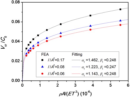
Fig. 11Vcr/C0 vs. ρA/(ET2) for different I/A2 a) and b) Vcr/C0 vs. I/A2 for different ρA/(ET2)
a)
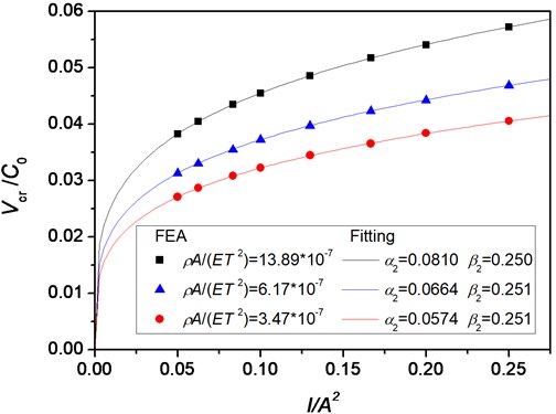
b)
The relationship between and for three sets of values of is illustrated in Fig. 11(a). It can be found that increases as increases for a particular value of . This relation can be fitted by a power law:
where and are fitting parameters. The fitting results of and corresponding to the three sets of values of are also shown in Fig. 11(a). For different , is almost constant, which is approximately equal to 0.25.
Similarly, the relationship between and for three sets of values of is illustrated in Fig. 11(b). For a particular value of , increases with the increase of . A power function is also selected to fit the relationship between and :
where and are fitting parameters. From Fig. 11(b), it is found that is very close to 0.25 for different .
According to these understandings, for simplicity, the fitting function of is taken as:
where is a fitting parameter. Fitting all above finite element results, we obtain 2.36. Thus, we have:
where is the gyration radius of the beam cross-section, which is equal to . Therefore, the critical velocity is affected by the speed of elastic wave, the gyration radius and the pulse duration. These three parameters characterize the material, structural and load properties, respectively.
According to Ref. [1], the spatial interval between the positive and the negative peak of the air pressure pulse, , is constant for a particular type of trains. In our finite element model, this spatial interval is equal to . When the velocity of moving pulse reaches the critical velocity, we have . In this critical situation, substituting into Eq. (8) yields:
The critical velocity decreases as the spatial interval grows when the gyration radius and the speed of elastic wave are constant. The spatial interval is strongly dependent on the shape of the fore- and after-bodies of trains [1]. The designers of high-speed train may make the critical velocity meet the safety standard by modifying the shape of the fore- and after-bodies of trains.
4. Conclusions
The dynamic response of a beam to a moving single sinusoidal pulse is investigated by using finite element method with ABAQUS/Explicit code. For a particular pulse duration, there is a critical velocity at which the average value of maximal equivalent stress reaches its maximum value. The critical velocity decreases as the pulse duration increases, but the average value of maximal equivalent stress at the critical velocity increases as the pulse duration grows. The position of maximum degree of bending appears in the first peak of beam deflection, then in the first valley, then in the second peak, and so on. With dimensionless analysis, the empirical formulas of critical velocity and the factors influencing the critical velocity are obtained. The amplitude of moving pulse and the Poisson’s ratio have no effect upon the critical velocity. The critical velocity is only affected by the speed of elastic wave, the gyration radius of the cross-section and the pulse duration. These influencing parameters characterize the material, structural and load properties.
In the present study, the amplitude of moving pulse keeps constant for any velocity of moving pulse. As the model used is linear, the maximal equivalent stress obtained can be directly amplified with a factor which is the ratio of the objective amplitude of moving pulse to the one used above. For example, one may consider the fact that the amplitude of moving pulse produced by trains passing each other is proportional to the square of the speed of trains [1]. This presents a method to consider the influence of the speed of trains on the amplitude pressure of moving pulse. As the velocity of moving pulse grows, the maximal equivalent stress in a train reaches a peak value at a certain velocity and then gradually increases. Thus, the passing train speed should not exceed a certain limit, which will be sensitive to the line intervals of rail traffic. For a predetermined line interval of rail traffic, the operational speed of trains when passing each other depends mainly on the structure intensity of train carriage. The optimization of the shape of train nose and the structural performances of carriage is suggested to increase the safe speed of trains.
This work may help to understand the mechanism of the dynamic response of trains when they pass each other. As trains run at high speed, the dynamic effect by the moving pulse when they pass each other becomes more important and needs to be further studied in the safety design and structure optimization of train carriage, due to the complexity of the train carriage structure.
References
-
Raghunathan R. S., Kim H. D., Setoguchi T. Aerodynamics of high-speed railway train. Progress in Aerospace Sciences, Vol. 38, Issues 6-7, 2002, p. 469-514.
-
Tian H. Q., Yao S., Yao S. G. Influence of the air pressure pulse on car-body and side-windows of two meeting trains. China Railway Science, Vol. 21, Issue 4, 2000, p. 6-12, (in Chinese).
-
Ozawa S. Aerodynamic forces on train. The Japan Society of Mechanical Engineers, 1990, p. 900-937, (in Japanese).
-
Fryba L. Vibration of solids and structures under moving loads. Third Edition, Thomas Telford Ltd., London, 1999.
-
Timoshenko S. P. Method of analysis of static and dynamic stresses in rails. Proc. Second International Congress for Applied Mechanics, Zurich, Switzer-land, 1927, p. 1-12.
-
Florence A. L. Traveling force on a Timoshenko beam. Journal of Applied Mechanics, Vol. 32, Issue 2, 1965, p. 351-359.
-
Chen Y. H., Huang Y. H. Dynamic characteristics of infinite and finite railways to moving loads. Journal of Engineering Mechanics – ASCE, Vol. 129, 2003, p. 987-995.
-
Sun L. Dynamic displacement response of beam-type structures to moving loads. International Journal of Solids and Structures, Vol. 38, Issues 48-49, 2001, p. 8869-8878.
-
Nechitailo N. V., Lewis K. B. Critical velocity for rails in hypervelocity launchers. International Journal of Impact Engineering, Vol. 33, Issues 1-12, 2006, p. 485-495.
-
Savin E. Dynamic amplification factor and response spectrum for the evaluation of vibrations of beams under successive moving loads. Journal of Sound and Vibration, Vol. 248, Issue 2, 2001, p. 267-288.
-
Adams G. G. Critical speeds and the response of a tensional beam on an elastic foundation to repetitive moving loads. International Journal of Mechanical Sciences, Vol. 37, Issue 7, 1995, p. 773-781.
-
Graff K. F. Wave Motion in Elastic Solids. Dover Publications, Inc., New York, 1991.
-
Kolsky H. Stress Wave in Solids. Clarendous Press, Oxford, 1953.
About this article

The financial supports from the National Basic Research Program of China (973 Program, Grant No. 2011CB711100), the National Natural Science Foundation of China (Project No. 11372307) and the Chinese of (Grant No. KJCX2-EW-L03) are acknowledged.
