Fuzzy-PID controller on ANFIS, NN-NARX and NN-NAR system identification models for cylinder vortex induced vibration

Mohammed, Mohammed Jawad; Mat Darus, Intan Z.

Journal of Vibroengineering

Browse Journal

Submit article

Published: 15 November 2014

Check for updates

Fuzzy-PID controller on ANFIS, NN-NARX and NN-NAR system identification models for cylinder vortex induced vibration

Mohammed Jawad Mohammed¹

Intan Z. Mat Darus²

¹Electromechanical Systems Department, University of Technology, Baghdad, Iraq

^{1, 2}Department of Applied Mechanics, Universiti Teknologi Malaysia, Johor Bahru, Johor, Malaysia

Corresponding Author:

Mohammed Jawad Mohammed

Cite the article Download PDF

Downloads 1320

Abstract

In this paper, Fuzzy-PID controller on nonlinear system identification models for cylinder due to vortex induced vibration (VIV) has been presented well. Nonlinear system identification models generated after extracting the input-output data from previous paper. The nonlinear model consisted into three methods: Neural Network (NN-NARX) based on the Nonlinear Auto-Regressive with External (Exogenous) Input, Neural Network (NN-NAR) based on the Nonlinear Auto-Regressive and Adaptive Neuro-Fuzzy Inference System (ANFIS). The work has been divided into two main parts: generating the system identification models to predict the system dynamic behavior and using Fuzzy-PID controller to suppress the cylinder vibration arising from the vortices. For system identification models, the best representation for NAR and NARX models has been chosen depend on two variables which are Number of hidden neurons (NE) and number of delay (ND) then using mean Square Error (MSE) to find the best model. Whereas, calculating the lowest MSE when the ND equal to 2 and the value of NE ranging 1-11 then fixing NE which is giving the lowest MSE and calculating it when the ND ranging 1-11. While, for ANFIS model the process consisted of find the lowest MSE at particular number of membership function (MF) with two inputs and generalized bell shape as a type of MF. For the second part, Fuzzy-PID used to attenuate the effect of vortices on the cylinder on the best representation for all methods. However, the consequences presented that the lowest MSE of NAR model equal 2.8452×10^-9 when the NE = 6 and ND = 4. While the best model of the NARX method recorded MSE = 1.2714×10^-9 at NE and ND equal to 8 and 2 respectively. Also, the lowest MES for ANFIS model recorded 2.5635×10^-13 when the MF equal to 2 for input and output. From another hand, Fuzzy-PID controller has been succeeded to reduce the vortex induced vibration on cylinder for all models but particularly on ANFIS model.

1. Introduction

In offshore engineering, vortex induced vibration (VIV) is one of the most important phenomena of the marine engineering designers for being the main reason for the failure occurs in the structures exposed to a stream of water or air for many applications such as oil transportation pipelines [1-2].

It is happen when the cylinder position being perpendicular with the flow direction which leads to the vibration of the cylinder transversely go up and down due to the force formed by the vortices behind the structure which leads to large damage especially when the vortex shedding frequency locks to the natural frequency of the structures [3-4].

From previous papers, forces formed by the vortices that can be divided into two main sections depend on the direction of the cylinder motion. If the vibrating cylinder toward cross flow direction ( $Y$ axis), it is called lift force while if the cylinder vibrates toward inline flow direction, it is called drag force ( $X$ axis) [5-6].

To avoid this trouble, there are three ways used in the history of the VIV phenomenon to suppress the cylinder vibration which are: active, passive and semi active or semi passive vibration control. The first way depends on using actuators and sensors during from feedback loop. This way considered the cheapest, most efficient and the most widely used at the present time [7]. The second way depends on increasing the section area of the cylinder during from adding springs and dampers while the last way depends on combine between active and passive ways like in the suspension systems.

Nowadays, there are several strategies used to minimize the vibration caused by vortices as one of the ways of using the active vibration method such as create the perturbation on the surface of the cylinder [8], use boundary layer control technique [9] and finally using the rotary cylindrical actuator on the body [10].

From the other hand, system identification one of the important way in industrial applications such as fault diagnosis and machine monitoring to study the dynamic performance of the system especially when the intended understanding the mathematical relationships between the input and output signals of a physical system for modeling, control (dynamic specifications of control) and prediction (prediction of commodities and expectation of energy load) Also, few papers studied the VIV during from representation the behavior of the system by using system identification methods and then using the controller in this application. The first endeavor was by Shaharuddin and Mat Darus (2012) which used PID controller on the Least Square (LS) and Recursive Least Square (RLS) as a linear system identification model by Shaharuddin and Mat Darus (2013) [11], then comparison between ANFIS, LS and RLS models to represent the system [12] and recently using Fuzzy-PID controller on RLS system identification model in this application by Shaharuddin and Mat Darus (2013) [13].

This paper consisted of four main parts: firstly, data collection from prior papers. Secondly, represent the models by using nonlinear Neural Network based on NAR, NARX and ANFIS system identification methods. Thirdly, use Fuzzy-PID controller on the models and finally validation and discussion the results.

2. Data collection

Data has been collected from previous researches by Shaharuddin and Mat Darus [12-13] which are consisted of 33000 data for the input and output from accelerometers A and B during the vibration of the cylinder in cross-flow direction by using water current flow inside the basin. The experimental setup included of using miniature basin (3 m, 1.5 m and 1 m as a length, width and depth respectively) in the laboratory of the Universiti Teknologi Malaysia. While the cylindrical pipe has been made from aluminum and fully immersed inside the basin with dimensions 50 mm and 1110 mm as a diameter and length respectively. The cylinder has been supported by four springs to allow it to vibrate in cross flow only by using water pump strongly 3 hp as shown in Fig. 1. Two accelerometers (A and B) have been used to collect the input and output data by using Data Acquisition (DAQ) National Instruments as shown in Fig. 2. The accelerometer A represents the detected input data which put it in the direction of water flow while the accelerometer B represents the observed output for system identification which put it in the mid of the cylinder. Table 1 and shown the cylinder properties of the experimental setup and Fig. 3 shown the relationship between the amplitude and the time for the input and output data.

Fig. 1Experimental setup model for the system [12-13]

Table 1Obtained parameters [12-13]

Parameter	Symbol	Value	Unit
Cylinder diameter	$D$	50	mm
Cylinder length	$L$	1110	mm
Aspect ratio	$L / D$	22.2	Dimensionless
Cylinder mass	$m$	2.95	kg
Mass ratio	$m^{*}$	1.18	Dimensionless
Natural frequency in water	$f_{w}$	1.11	Hz
Damping ratio in water	$ζ$	0.1007	Dimensionless
System stiffness	$k$	265.34	N/m

Fig. 2Data acquisition (DAQ) national instruments [12-13]

Fig. 3a) Data obtained for the input and b) the output for the system [12-13]

a)

b)

3. System identification

System identification used to create the transfer function or equivalent model for the linear and nonlinear system from estimated data [14]. In this work, system identification model has been used to generate the model during from product the dynamic behavior of the system by using nonlinear methods which are: NN-NARX, NN-NAR and ANFIS models.

3.1. Nonlinear auto-regressive model (NAR)

It is one of the nonparametric algorithms used to predict the output model from experimental work of actual output data. The equations of the method can be summarized as follows [15]:

1

y (t) = \frac{ξ (z^{- 1})}{A (z^{- 1})},

where:

2

A (z^{- 1}) = 1 + a_{1} z^{- 1} + \dots + a_{n} z^{- n} .

After neglecting the noise error $ξ (t)$ and substitute $A (z^{- 1})$ the equation above became:

3

y (t) = f [y (t - 1), \dots ., y (t - n_{a})],

where $n_{a}$ represents to the previous output and $f$ represents the nonlinear methods by using intelligent ways such as Neural Network.

3.2. Nonlinear auto-regressive external input model (NARX)

It is one of the nonparametric algorithms used to predict the output model from experimental work of actual input and output data. The equations of the method can be summarized as follows [16]:

4

y (t) = \frac{B (z^{- 1})}{A (z^{- 1})} u (t) + \frac{ξ (z^{- 1})}{A (z^{- 1})},

where:

5

A (z^{- 1}) = 1 + a_{1} z^{- 1} + \dots + a_{n} z^{- n},

6

B (z^{- 1}) = b_{0} + b_{1} z^{- 1} + \dots + b_{n} z^{- (n - 1)} .

After neglecting the noise error $ξ (t)$ and substitute $A (z^{- 1})$ the equation above became:

7

y (t) = f [y (t - 1), \dots ., y (t - n_{a}), u (t - n_{k}), u (t - n_{k} - n_{b} + 1)],

where $n_{a}$ and $n_{b}$ represent to the previous input output respectively. $n_{k}$ reprsesnt the system delay and $f$ represents the nonlinear methods by using intelligent ways such as Neural Network.

3.3. Neural network time series

This process depends on two important parameters to create the nonlinear model. The first parameter called number of hidden neurons (NE) while the second parameter called number of delay which depends on number of input and output from the experimental work enters to the system sequentially. Depend on Fig. 4, the process to find the output value by using neural network can be specified during from calculating the hidden and output layers equations. Whereas, for hidden layer:

8

v_{1} = x_{1} w_{11} + x_{2} w_{12} + y_{1} w_{13} + y_{2} w_{14} + b_{1},

9

v_{2} = x_{1} w_{21} + x_{2} w_{22} + y_{1} w_{23} + y_{2} w_{24} + b_{2},

then:

10

f_{1} = \frac{1}{1 + e^{{- v}_{1}}},

11

f_{2} = \frac{1}{1 + e^{{- v}_{2}}},

where $x_{1}, x_{2}$ refer to the actual input and $y_{1}, y_{2}$ refer to the actual output data. $w_{11}$ , $w_{12}$ , $w_{13}$ , $w_{14}$ , $w_{21}$ , $w_{22}$ , $w_{23}$ , $w_{24}$ refer to the weights of hidden layer. $b_{1}$ , $b_{2}$ refer to the bias weights for hidden layer. $v_{1}$ , $v_{2}$ refer to the summation values for hidden layer. $f_{1}$ , $f_{2}$ refer to the final values for hidden layer.

Fig. 4Neural network architecture

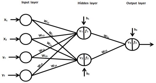
While the final equation for Neural Network Output layer:

12

v_{3} = f_{1} w_{31} + f_{2} w_{32} + b_{3},

13

f_{3} = \frac{1}{1 + e^{{- v}_{3}}},

where $w_{31}$ , $w_{32}$ refer to the weights of output layer while $b_{3}$ refers to the bias weights for output layer. $v_{3}$ refers to the summation values for output layer while $f_{3}$ refers to the final values for neural network.

3.4. Adaptive neuro-fuzzy inference system (ANFIS)

One of the nonlinear system identification models depends on neural network (NN) and fuzzy logic (FC) fundamentals to create the model. The aim of this method is to integrate the preferable specifications for both methods (FC and NN) where from fuzzy logic: impersonation of the previous knowledge into a group of constraints to minimize the optimization search domain while from NN: Adaptation of back propagation for network structure to automate FC tuning. According to the Fig. 5, a rule set for the system can be written [17]:

– If ( $x_{1}$ is $A_{1}$ ) and ( $x_{2}$ is $B_{1}$ ) then $f_{1} = p_{1} x_{1} + q_{1} x_{2} + r_{1}$ ;

– If ( $x_{1}$ is $A_{2}$ ) and ( $x_{2}$ is $B_{2}$ ) then $f_{2} = p_{2} x_{1} + q_{2} x_{2} + r_{2}$ .

Fig. 5ANFIS architecture

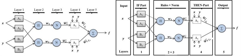
Based on to the ANFIS structure, $O_{l, i}$ is the output for layers. Whereas $i_{t h}$ is the output of the node in $l_{t h}$ layer [18]. Whereas, the objective for the first layer is to estimate the MF value for premise parameter as shown in equations below:

14

O_{1, i = 1,2} = μ_{A_{i}} (x_{1}),

15

O_{1, i = 3,4} = μ_{B_{i - 2}} (x_{2}),

where $A$ refers to the linguistic label and the output for this layer is:

16

μ_{A i} (x_{1}) = \frac{1}{1 + {|\frac{x_{1} + c_{i}}{a_{i}}|}^{2 b}} .

While, the objective for the second layer is for firing strength of the rule and the output for this layer is:

17

O_{2, i = 1,2} = ω_{i} = μ_{A_{i}} (x_{1}) . μ_{B_{i}} (x_{2}) .

Then, the objective for the third layer is for normalizing the firing strength for all rules and the output for this layer is:

18

O_{3, i} = {\bar{w}}_{i} = \frac{w_{i}}{w_{1} + w_{2}} .

While, objective for the fourth layer is to evaluate the Consequent Parameters and the output for this layer is:

19

O_{4, i} = {\bar{w}}_{i} f_{i} = {\bar{w}}_{i} (p_{i} x_{1} + q_{i} x_{2} + r_{i}) .

Finally, the objective for fifth layer is to find the overall output process which is:

20

O_{5,1} = \sum_{i} {\bar{w}}_{i} f_{i} = \frac{\sum_{i} w_{i} f_{i}}{\sum_{i} w_{i}} .

3.5. Validation technique

In this paper, MSE technique has been used to validate from the system identification results and this technique depends on the evaluation for actual and predictive output. The algorithm can be specified [19]:

21

ε (t) = \frac{1}{N} \sum_{t = 1}^{N} y (t) - \hat{y} {(t)}^{2},

where $y (t)$ is the actual output and $\hat{y} (t)$ is the predicted output.

4. Self-tuning Fuzzy-PID controller (FPID)

One of the important controllers used to study the performance for the linear and nonlinear model in this paper, FPIC controller has been used to control on the cylinder vibration caused by VIV after obtaining the data from prior papers. The process has been included many parts.

4.1. FPID structure

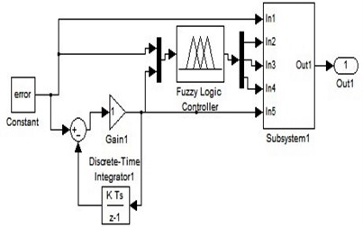
PID parameters ( $K_{I}$ , $K_{P}$ and $K_{D}$ ) have been tuned depend on the heuristic method to get the lower vibration for the cylinder. The effect of these parameters has been discussed from pervious paper [20]. The input of FPID controller arisen based on the error $(e)$ which referred to the value between the desired reference and the output of the system and the variation of the error $(\dot{e})$ which refereed to the derivative of error as shown in Figs. 6 and 7.

The control feedback loop has been used to compare between the input step reference ( $r$ ) with the output for the system after generating the models (NN-NAR, NN-NARX and ANFIS) by using nonlinear system identification method. The input of Fuzzy control consisted of two inputs (error and error derivative) in discrete time system to describe the nonlinear system accurately and three output which represented the PID parameters.

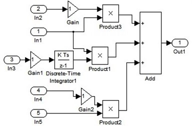
Fig. 6Input and output connection for Fuzzy controller

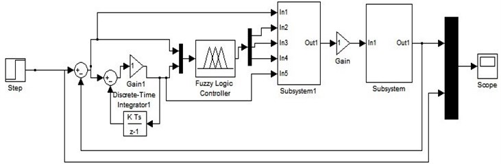
Fig. 7PID and FPID system block diagram

4.2. Fuzzification

Fig. 8Input and output intervals for fuzzification

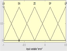
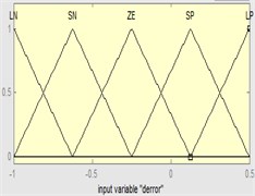
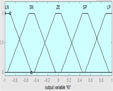
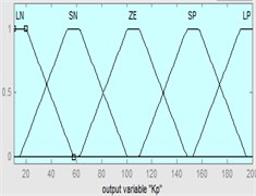
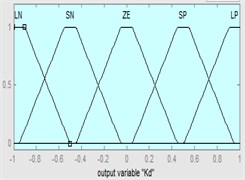
Triangle shapes for MF have been used for the input and trapezoidal shapes for the output of Fuzzy controller because of its very common for previous papers [21]. Different intervals used for the input and output of FPID controller depends on the type of model. Where for NN-NAR model the interval for the $(e)$ and $(\dot{e})$ ranged [1, 1.6] while the interval of the output ranged [0, 0.4] for $K_{I}$ , [–1, 1] for $K_{P}$ and [–0.4, 0.3] for $K_{D}$ . For NN-NARX model the interval of the $(e)$ and $(\dot{e})$ ranged [–1.5, 1.5] while the interval for the output ranged [–10, 10] for $K_{I}$ , [–5, 5] for $K_{P}$ and [–0.4, 0.4] for $K_{D}$ . Also, for ANFIS model the interval of the $(e)$ and $(\dot{e})$ ranged [–1, 0.5] while the interval for the output ranged [10, 200] for $K_{I}$ , [–1, 1] for $K_{P}$ and [–1, 1] for $K_{D}$ as shown in Fig. 8. Also, large positive (LP), small positive (SP), zero (ZE), large negative (LN) and small negative (SN) was the linguistic descriptions for the controller.

4.3. Rule-base

Generally, it’s important to find the suitable rules to improve the system performance. The Fuzzy control form for the rule set is:

$R_{k}$ : if refers $A_{i}$ and $\dot{e}$ refers $B_{j}$ then $K_{P}$ refers $C_{i j}$ , $K_{I}$ refers $D_{i j}$ and $K_{D}$ refers $E_{i j}$ . Where, the $R_{k}$ is the condition for fuzzy control while $A_{i}$ refers to the error for fuzzy set and $B_{j}$ refers to the change of error for fuzzy set.

Five linguistic descriptions has been used for the both input of fuzzy control which resulted 25 rules for the outputs as shown in Table 2 [22].

Table 2Fuzzy controller rule set

Parameters $K_{I}$ , $K_{P}$ and $K_{D}$		Error
Parameters $K_{I}$ , $K_{P}$ and $K_{D}$		LN	SN	ZE	SP	LP
Variation of error	LN	LN	LN	SN	SN	ZE
	LS	LN	LN	SN	ZE	SP
	ZE	SN	SN	ZE	SP	SP
	SP	SN	ZE	SP	SP	LP
	LP	ZE	SP	SP	LP	LP

4.4. Defuzzification

The aim of this process is to convert the linguistic variables to the classic or crisp outcomes. Min and max methods have been used for and or method respectively while min operator chosen for implication method and center of gravity method used as defuzzification process because of this method considered most prevalent from the physical side [23].

5. Obtained results and discussions

5.1. System identification for NN-NAR and NN-NARX models

In this work, 33000 input and output data have been used to create the model which divided into three parts: 32100 for training, 4950 for validating and 4950 for testing. The process for these methods consisted of two portions to find the best model to represent the system. Firstly, calculate the lowest MSE for NN-NAR and NN-NARX models when the ND = 2 and NE ranged 1-11 neurons. Secondly, calculate the lowest MSE for the best case from first step with different ND which ranged 1-11.

According to Tables 3 and 4, the lowest MSE for NN-NARX model has been recorded 1.2714×10^-9 at NE = 8 and at ND = 2 while the lowest MSE remained at same value when NE fixed at 8 with different ND. Fig. 9 appeared the amplitude and the error values with time.

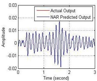
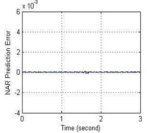
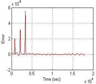
According to Tables 5 and 6, the lowest MSE for NN-NAR model has been recorded 6.6542×10^-9 at NE = 6 and at ND = 2 while the lowest MSE recorded 2.8452×10^-9 when NE fixed at 6 and ND = 4. Fig. 10 appeared the amplitude and the error values with time.

Table 3Mean square error for NARX model at number of delay 2

NE	MSE for training	MSE for validating	MSE for testing	MSE overall
1	7.06994×10^-7	7.03911×10^-7	7.30382×10^-7	7.1048×10^-7
2	1.51825×10^-7	1.46421×10^-7	1.63488×10^-7	1.5353×10^-7
3	2.51148×10^-9	2.53456×10^-9	2.49492×10^-9	3.2278×10^-9
4	2.25323×10^-8	2.10880×10^-8	2.24574×10^-8	2.2795×10^-8
5	1.90786×10^-9	1.88947×10^-9	1.91908×10^-9	2.2781×10^-9
6	2.33170×10^-8	2.42179×10^-8	2.39115×10^-8	2.4056×10^-8
7	8.42986×10^-8	8.52992×10^-8	8.58115×10^-8	8.5672×10^-8
8	4.7337×10^-10	4.7219×10^-10	4.7699×10^-10	1.2714×10^-9
9	3.27642×10^-9	3.31040×10^-9	3.41665×10^-9	4.0278×10^-9
10	6.28938×10^-9	6.58235×10^-9	6.65887×10^-9	6.7772×10^-9
11	1.60514×10^-8	1.62700×10^-8	1.75777×10^-8	1.6682×10^-8

Table 4Mean square error for NARX model at number of hidden neuron 8

ND	MSE for training	MSE for validating	MSE tested	MSE overall
1	1.2692×10^-8	1.2709×10^-8	1.3011×10^-8	1.3078×10^-8
2	4.7337×10^-10	4.7219×10^-10	4.7700×10^-10	1.2714×10^-9
3	2.3379×10^-10	2.2933×10^-10	2.3540×10^-10	1.3273×10^-9
4	6.0016×10^-9	6.0448×10^-7	5.9680×10^-7	6.4521×10^-9
5	1.8549×10^-8	1.8502×10^-8	1.8931×10^-8	1.9537×10^-8
6	3.0966×10^-8	3.1253×10^-8	1.0954×10^-8	3.2182×10^-8
7	3.3785×10^-8	3.6127×10^-8	3.4293×10^-8	3.4956×10^-8
8	1.3636×10^-9	1.3966×10^-9	1.3686×10^-9	2.8229×10^-9
9	2.0855×10^-9	2.0098×10^-9	1.9893×10^-9	3.7473×10^-9
10	2.7858×10^-9	2.7113×10^-9	2.8606×10^-9	2.8790×10^-8
11	7.7023×10^-9	7.7061×10^-9	8.0669×10^-9	8.9183×10^-9

Table 5Mean square error for NAR model at number of delay 2

NE	MSE for training	MSE for validating	MSE tested	MSE overall
1	1.21865×10^-8	1.23348×10^-8	1.47379×10^-8	1.3618×10^-8
2	4.69192×10^-7	4.44050×10^-7	5.13385×10^-7	4.7309×10^-7
3	6.160202×10^-8	6.42999×10^-8	6.11500×10^-8	6.2567×10^-8
4	2.95893×10^-7	2.89721×10^-7	3.12913×10^-7	2.9778×10^-7
5	1.01116×10^-8	1.02313×10^-8	1.00981×10^-8	1.0532×10^-8
6	5.82502×10^-9	5.97741×10^-9	5.76880×10^-9	6.6542×10^-9
7	9.52759×10^-8	8.19346×10^-8	1.00706×10^-7	9.4854×10^-8
8	7.40069×10^-9	6.37130×10^-9	6.98316×10^-9	7.7572×10^-9
9	2.54389×10^-8	2.79919×10^-8	2.74169×10^-8	2.9366×10^-8
10	1.45673×10^-8	1.48914×10^-8	1.48435×10^-8	1.6209×10^-8
11	9.78359×10^-8	8.76832×10^-8	9.03277×10^-8	9.5864×10^-8

Table 6Mean square error for NAR model at number of hidden neuron 8

ND	MSE for training	MSE for validating	MSE tested	MSE overall
1	1.43914×10^-7	3.98960×10^-7	3.99911×10^-7	4.0290×10^-7
2	5.82502×10^-9	5.97741×10^-9	5.76880×10^-9	6.6542×10^-9
3	3.47933×10^-9	3.43426×10^-9	3.52902×10^-9	4.1027×10^-9
4	9.78777×10^-10	9.78197×10^-10	9.87599×10^-10	2.8452×10^-9
5	1.04383×10^-8	1.03251×10^-8	1.04343×10^-8	1.1098×10^-8
6	5.04420×10^-9	4.97154×10^-9	4.94863×10^-9	6.3538×10^-9
7	4.52312×10^-8	4.65865×10^-8	4.73918×10^-8	4.7095×10^-8
8	7.65045×10^-9	7.90956×10^-9	7.81632×10^-9	8.8763×10^-9
9	1.84328×10^-9	1.87072×10^-9	1.81564×10^-9	3.0986×10^-9
10	7.23659×10^-8	7.55279×10^-8	7.30517×10^-8	7.3678×10^-8
11	1.37098×10^-8	1.21062×10^-8	1.32999×10^-8	1.4201×10^-8

Fig. 9a) Relationship between the amplitude and b) error with time of NN-NARX model

a)

b)

Fig. 10a) Relationship between the amplitude and b) error with time of NN-NAR model

a)

b)

5.2. System identification for ANFIS model

Five steps have been used to produce the ANFIS system identification model which is: firstly, use two inputs for the model as shown in Fig. 11 after selecting 15000 data for training and 18000 data for testing as shown in Table 7. Secondly, specify [2, 2] as a number of MF and generalized bell shape as a type of MF. Thirdly, create the Fuzzy model. Fourthly, specify the tolerance and epoch numbers to create the ANFIS mode and finally evaluate the system.

Fig. 11ANFIS architecture

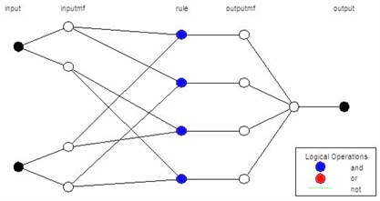
Table 7ANFIS information

ANFIS information	Values
Linear parameter number	4
Nonlinear parameter number	12
Total parameter number	24
Training number	15000
Checking number	18000

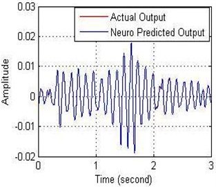
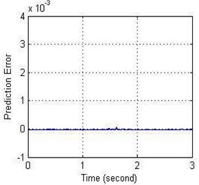
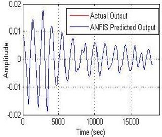
According to Fig. 12, the results shown that the lowest MSE recorded 2.5635×10^-13. That’s mean; the ANFIS model was the most accurate prediction of the dynamic response of the system from other models.

Fig. 12a) Relationship between the amplitude and b) error with time of ANFIS model

a)

b)

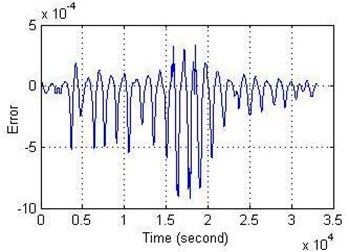
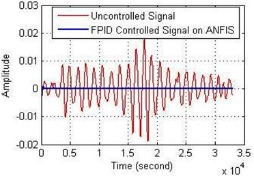
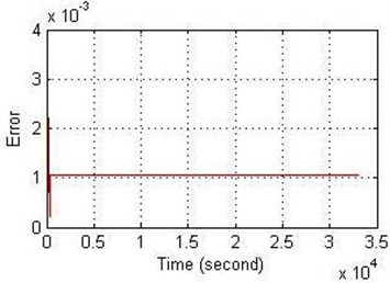
5.3. FPID controller for NN-NAR, NN-NARX and ANFIS models

FPID controller has been used to study the performance of the controller to suppress the cylinder vibration in marine application which it’s caused by vortex induced vibration after generating the mathematical models by using nonlinear system identification methods which consisted of three types: NN-NAR, NN-NARX and ANFIS models.

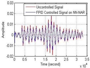
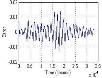
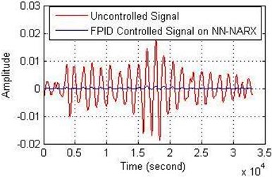
The structure of the controller for all models has been included two inputs and three outputs. According to the Figs. 13, 14 and 15, the results shown that the best attenuation of VIV on the cylinder is when it used FPID controller on the ANFIS model. Also, FPID controller on NN-NARX has been succeeded to reduce the vibration on the cylinder while the FPID controller on NN-NAR has been bit suppression on the cylinder and this result was not unsatisfactory.

Fig. 13FPID controller performance on NN-NAR for: a) the amplitude and b) the error

a)

b)

Fig. 14FPID controller performance on NN-NARX for: a) the amplitude and b) the error

a)

b)

Fig. 15FPID controller performance on ANFIS for: a) the amplitude and b) the error

a)

b)

6. Conclusions

FPID discrete time controller has been used to suppress the VIV on the pipe cylinder which it represented by using three nonlinear system identification models which are: NN-NAR, NN-NARX and ANFIS models. Firstly the ANFIS model has been recorded the lowest MSE = 2.5635×10^-13 when the number of input equal 2 and number of MF = [2, 2] with generalized bell shape. Then, NN-NARX model recorded MSE = 1.2714×10^-9 at NE and ND equal to 8 and 2 while, NN-NAR model recorded MSE = 2.8452×10^-9 when the NE = 6 and ND = 4. The second step has been included using FPID controller on the three models to get the best suppression in the cylinder in marine engineering applications. FPID controller on ANFIS model has been recorded the best suppression from other model. Also, FPID controller on NN-NARX model has been succeeded to suppress the effect of VIV while the FPID controller on NN-NAR has been bit suppression on the cylinder and this result was not unsatisfactory

References

Williamson C., Govardhan R. Vortex-induced vibrations. Journal of Fluid Mechanics, Vol. 36, Issue 1, 2004, p. 413-455.

Search CrossRef
Morse T., Williamson C. Prediction of vortex-induced vibration response by employing controlled motion. Journal of Fluid Mechanics, Vol. 634, 2009, p. 5-39.

Search CrossRef
Wanderley J., Levi C. Vortex induced loads on marine risers. Journal of Ocean Engineering, Vol. 32, Issue 11-12, 2005, p. 1281-1295.

Search CrossRef
Song J., Lu L., Teng B., Park H., Tang G., Wu H. Laboratory tests of vortex-induced vibrations of a long flexible riser pipe subjected to uniform flow. Journal of Ocean Engineering, Vol. 38, Issue 11-12, 2011, p. 1308–1322.

Search CrossRef
Bearman P. Circular cylinder wakes and vortex-induced vibrations. Journal of Fluids and Structures, Vol. 27, Issue 5-6, 2011, p. 648-658.

Search CrossRef
Mendonça Bimbato A., Alcântara Pereira L., Hiroo Hirata M. Suppression of vortex shedding on a bluff body. Journal of Wind Engineering and Industrial Aerodynamic, Vol. 121, 2013, p. 16-28.

Search CrossRef
Rémi B., David L. Active control of a reduced scale riser undergoing vortex-induced vibration. Journal of Offshore Mechanics and Arctic Engineering, Vol. 135, Issue 1, 2013, p. 1-5.

Search CrossRef
Cheng L., Zhou Y., Zhang M. Controlled vortex-induced vibration on a fix-supported flexible cylinder in cross-flow. Journal of Sound and Vibration, Vol. 292, Issue 1-2, 2006, p. 279-299.

Search CrossRef
Korkischko I., Meneghini J. Suppression of vortex-induced vibration using moving surfaceboundary-layer control. Journal of Fluids and Structures, Vol. 34, Issue 5, 2013, p. 259-270.

Search CrossRef
Rémi B., David L. Flow-induced vibrations of a rotating cylinder. Journal of Fluid Mechanics, Vol. 740, 2014, p. 342-380.

Search CrossRef
Shaharuddin N., Mat Darus I. Active vibration control of marine riser. IEEE International Conference on Control, Systems and Industrial Informatics, 2012, p. 114-119.

Search CrossRef
Shaharuddin N., Mat Darus I. System identification of flexibly mounted cylindrical pipe due to vortex induced vibration. IEEE International Symposium on Computer and Informatics, 2013, p. 30-34.

Search CrossRef
Shaharuddin N., Mat Darus I. Fuzzy-PID control of transverse vibrating pipe due to vortex induced vibration. IEEE International Conference onComputer, Modelling and Simulation, 2013, p. 21-26.

Search CrossRef
Eke R., Mat Darus I., Sahlan S. Development of MATLAB GUI application for system identification (SID) of beam structure. WSEAS International Conference on Instrumentation, Measurement, Circuits and Systems, 2013, p. 147-152.

Search CrossRef
Syrmos V. Nonlinear system identification and fault detection using hierarchical clustering analysis and local linear models. Mediterranean Conference on Control and Automations, 2007, p. 1-6.

Search CrossRef
Peng H., Ozaki T., Toyoda Y., Shioya H., Nakano K., Haggan-Ozaki V., Mori M. RBF-ARX model-based nonlinear system modeling and predictive control with application to a NOx decomposition process. Journal of Control Engineering Practice, Vol. 12, Issue 2, 2004, p. 191-203.

Search CrossRef
Jang J. ANFIS: adaptive-network-based fuzzy inference system. IEEE Transaction Systems, Vol. 23, Issue 5-6, 1993, p. 665-685.

Search CrossRef
Jang J., Sun C. Neuro-fuzzy modeling and control. Proceeding of IEEE, Vol. 83, Issue 3, 1995, p. 378-406.

Search CrossRef
Tavakolpour A., Mat Darus I., Tokhi O., Mailah M. Genetic algorithm-based identification of transfer function parameters for a rectangular flexible plate system. Journal of Engineering Applications of Artificial Intelligence, Vol. 23, Issue 8, 2010, p. 1388-1397.

Search CrossRef
Tavakolpour A., Mat Darus I., Mailah M. Active vibration control of a rectangular flexible plate structure using high gain feedback regulator. International Review of Mechanical Engineering, Vol. 3, Issue 5, 2009, p. 579-587.

Search CrossRef
Ranjbar B., Dashti G., Omidvar A., Mahmoodi J., Karbasi H. Design PID tuning Fuzzy controller forhighly nonlinear system. International Journal of Modern Education and Computer Science, Vol. 6, 2014, p. 54-63.

Search CrossRef
Zulfatman, Rahmat M. Application of self-tuning Fuzzy PID controller on industrial hydraulic actuator using system identification approach. International Journal on Smart Sensing and Intelligent Systems, Vol. 2, Issue 2, 2009, p. 246-261.

Search CrossRef
Lee C. Fuzzy logic in control systems: Fuzzy logic controllers – part 1. IEEE Transaction on Systems, Vol. 20, Issue 2, 1990, p. 408-418.

Search CrossRef

About this article

Received

11 May 2014

Accepted

07 September 2014

Published

15 November 2014

Keywords

nonlinear system identification

vortex induced vibration

fuzzy-PID controller

Acknowledgements

Ministry of Education (MOE) and Universiti Teknologi Malaysia (UTM) for Research University Grant (Vote No. 04H17) and for acknowledgement of University of Technology (Iraq).

This is an open access article distributed under the Creative Commons Attribution License, which permits unrestricted use, distribution, and reproduction in any medium, provided the original work is properly cited.