Identification of second-order kernels in aerodynamics

1. Introduction

Nowadays, the most powerful and sophisticated tools for predicting nonlinear unsteady aerodynamic characteristics are being developed in the field of computational fluid dynamics (CFD). The application of CFD codes involves, in general, the application of the discretized Navier-Stokes (NS) equations. For the case where flow-induced nonlinearities at transonic flight conditions are significant in the aerodynamic response, time integration of the nonlinear equations is necessary. Using CFD codes the computational costs become prohibitively expensive, both in terms of CPU costs and turnaround time. This can be on the order of hours or days, depending on the user’s computer, the complexity of the structure model and the condition of flow field. This disadvantage really restricts its applications combining with other disciplines; especially in the design of aircraft control systems and aeroelastic systems.

Attempts to address this problem include the development of transonic indicial responses and impulse responses. Another approach to reduce the computational cost of CFD codes is to linearize the response about a nonlinear steady-state condition, obtain a linear state-space representation of the system of interest. If a linearized aerodynamic model from a CFD model is preferred, the method of the step or pulse input can be applied. In the identification fields, other methods or manners can also be employed. For examples: wavelet approximation and scale transformation, POD method, Volterra variational approach, neural network, incremental harmonic balance methods for airfoil flutter, etc [1-5].

The discrete impulse input was first suggested by Silva [6] in his dissertation to identify the Volterra kernels of nonlinear aerodynamic systems using the CFL3D code. Three conditions should be satisfied that 1) the kernels, input function, and subsequently, the output function are real-valued functions; 2) the system is causal; 3) the system is time invariant. Continuing on the work of Silva, Raveh generated a reduced-order model (ROM) by using step responses as the ROM’s kernels, for evaluation of generalized aerodynamic force (GAF) matrices. Raveh’s work [7] showed a better accuracy as compared to the Volterra ROM based on impulse response. CFD analysis shows that a step response, in contrast with an impulse method, is less prone to numerical problem and the identification of step-type kernels is less sensitive to such error. Raveh’s work also showed that it was difficult to identify the second-order Volterra kernels correctly for a particular aerodynamic problem.

There are mainly two reasons listed below:

a) The numerical limitations restrict the impulse/step maximum input amplitude and the minimum time step which can be accurately handled by the CFD numerical scheme. Whichever a pulse-response or a step-response method is used, the data needed for the identification of second-order kernel function is huge.

b) Based on the second-order ROM the second-order kernel function is difficult to be identified correctly.

In this paper, we first set up a third-order Volterra ROM to improve the accuracy of identification and then try to identify the second-order kernel function by using an alternative method, called Chebyshev expansion method. This identification technique does not strongly rely on the entire input and output data produced by CFD simulation. That means a colossal waste of time can be saved.

In Section 2, we briefly introduce the conceptions of Chebyshev polynomials, Volterra series and discrete impulse input. Next, we introduce first- and second-order ROM respectively. In Section 3, we put forward to the third-order ROM. Finally, we propose the identification method of Chebyshev polynomials. A CFD numerical scheme is employed to compute the aerodynamic forces of NACA0012 airfoil as the data for identification in transonic flow.

2. Preliminaries

3. Third-order ROM

As mentioned in the section of introduction, the second-order kernels sometimes can’t be identified correctly. In order to improve it, the higher-order ROM is proposed here. In a discrete system, it has the form below:

Similarly to the process of identification of second-order ROM, firstly let:

Next, feed them into Eq. (17). It follows:

where $\left|\right|u_i\left|\right|=2^{(i-1)}{\xi }_0$, $i=\text{1,}\text{2,}\text{3}$.

The first-order kernels and the components of the second-order kernels obtained by solving Eq. (19) have the forms below:

Feeding $u_T\left[n\right]={\xi }_0\cdot \delta \left[n\right]+{\xi }_0\cdot \delta [n-T+1]$ into Eq. (17), it follows:

where those third-order kernels’ terms are omitted since they are very smaller.

One can obtain the second-order kernels in the form as following:

where $\mathrm{}{h}_1\left[n\right]$, $h_2[n,n]$ are defined by Eqs. (20) and (21) respectively; $h_2[n-T+1,n-T+1]$ can be evacuated by a time shift of $h_2[n,n]$ according to the time-invariant hypothesis.

4. Example – nonlinear circuit

In the study of aerodynamics, the common methods include impulse-response method and step-response method. All the data for identification come from executing CFD numerical scheme. Before executing CFD code, the amplitude of an input must be chosen carefully whatever using an impulse-or step-response method since it may arise in different nonlinearities.

In order to identify the second-order kernels correctly, the third-order ROM is introduced here rather than the low-order ROMs studied by many other authors. One of them, Raveh [2], ever claimed in his paper that the problem to correctly identify the second-order kernels of nonlinear systems was quite difficult to a particular application.

For a simple nonlinear circuit system [1, 18], the governing equation is given below:

where $v$ is an input of voltage; $i$ is the output of the current around the circuit.

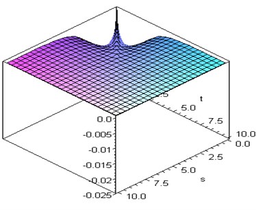
This nonlinear system can be remodeled by the second-order ROM as seen in Eq. (8). Using Eqs. (12) and (16), the first- and second-order kernels can be evacuated in an impulse-response method. They are presented in Figs. 1 and 2. As can be seen, the second-order kernel function is quite small in magnitude as compared to the first-order kernel function and goes to zero very quickly as well as the first-order kernel. Figs. 1 and 2 indicate that nonlinear effects are quite small.

Fig. 1First-kernel function of Riccati equation

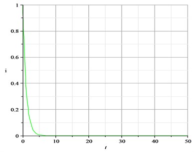
Fig. 2Second-kernel curve of Riccati equation

Using Chebyshev polynomials method for identification of the second kernel mentioned as in Eq. (3), the first thing is that we have to determine how many basis functions are properly chosen? Here, by testing after several times we find out that the number of basis functions is between 10 and 12. Hence, there are fifty-five coefficients need to be identified if we choose the number 10. Based on the orthogonal properties of Chebyshev polynomials, see in Eq. (2), all the coefficients can be evacuated. Substituting them into Eq. (3), one can obtain the second-order kernel function which is presented in Fig. 3.

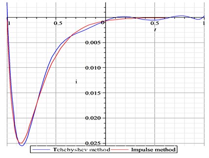
Let $s=$–1, the second-order kernels identified respectively by using an impulse-response method and Chebyshev polynomials method are presented in Fig. 4.

This example illustrates Chebyshev polynomials method can be used for deification of the second-order kernel function fully accurate in contrast to that identified by using an impulse-response method.

Fig. 3Second-kernel by Chebyshev polynomial

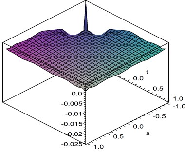
Fig. 4Comparison of second-kernels respectively by Chebyshev method and impulse method

5. Example- identification in transonic flows

During the last several decades there has been considerable interest in the accurate prediction of steady and unsteady transonic flows. Since transonic flow is inherently nonlinear and involves the formation of shock waves, accurate simulation of transonic flow requires the use of a nonlinear field equation, and for unsteady phenomena the solution needs to be time accurate. This paper employs a CFD (Computational Fluid Dynamics) code which is based on the Euler equation.

The two-dimensional Euler equations in Cartesian coordinates ($x$, $y$) can be written in non-dimensional conservative from as following [17]:

where $W=\left(\begin{array}{c}\rho \\ \rho u\\ \rho v\\ \rho E\end{array}\right)$ is the vector; $F=\left(\begin{array}{c}\rho U\\ \rho uU+p\\ \rho vU\\ U\left(\rho E+p\right)+x_{t}p\end{array}\right)$ and $G=\left(\begin{array}{c}\rho V\\ \rho uV\\ \rho vV+p\\ V\left(\rho E+p\right)+y_{t}p\end{array}\right)$ are the Cartesian components of the convective fluxes.

In the above $\rho$ is the fluid density, $u$ and $v$ are the $x$ and $y$ components of the fluid velocity, $E$ the total energy and $p$ is the pressure which is obtained from:

where $\gamma$ is the ratio of specific heats of the fluid.

The contravariant velocities $U$ and $V$ are defined by:

where $x_t$, $y_t$ are the grid speeds in the $x$ and $y$ directions respectively.

The Eq. (25) are discretized using a cell-centered finite volume method that transforms the partial differential equations into a set of ordinary differential equations that can be written as:

where $R_{i,j}\left(W\right)$ is the flux residual for the cell ($i$, $j$) that contains all the terms arising from the spatial discretization.

For the solution of the unsteady Euler equations, an implicit dual-time method can be employed. The initial conditions are chosen as the steady flow before the object moves. The boundary condition at the body is subject to the kinematic condition requiring the body to be impenetrable to the flow. Namely, the flow remains tangent to the body surface. The far-field boundary conditions are treated by the characteristic boundary method based on the Riemann invariants.

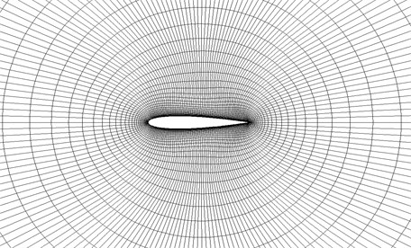
Fig. 5 is an O-type grid with 181×48 grid points for NACA0012. The steady inviscid comprssible flows about this airfoil is computed at Mach number $M_{\infty }=\text{0.8}$ and angle of attack $\alpha =\text{0}$ deg. The model has a NACA0012 airfoil secontion and a rectangular planform with a span of 0.8128 m and a chord of 0.2032 m. The rigid-body plunge mode consists only of vertical translation and the rigid-body pitch mode consists onlyof rotation about the mid-chord [19].

In aerodynamics, using Chebyshev polynomial method for the identification of kernels of the aerodynamic forces is seldom seen. Much more of its application can be found in theoretical research. The popular identification methods to a nonlinear system, say pulse- and step-type methods, highly rely on the entire data produced by executing CFD code again and again. As mentioned in the section of introduction, the cost of time-consumption is prohibitively expensive.

If the second-order kernels can not be identified correctly, the result of the aerodynamic forces of predicting can not be accurate and even badly wrong. Therefore, the third-order ROM is first suggested to be used here. The process of identification is presented in the section of third-order ROM above. The mainly advantages here are a) the first- and second-order kernels are steadily to be evacuated by Eqs. (20) and (23); b) Since the third-order kernels are not necessary to be identified, this model is appropriate to be applied; c) The high-order ROM helps to improve the identification accuracy of second-order kernels of nonlinear systems of interest.

Fig. 5Naca0012 airfoil and aerodynamic grid

In order to investigate the kernels' accuracy from the two models of ROMS of the second-order and the third-order, the first- and second-order kernels have been computed out respectively from Eqs. (20) and (23) in the third-order ROM and from Eqs. (12) and (16) in the second-order ROM, here ${\xi }_0=\text{0.05}$ is chosen and impulse-response method is employed.

The second-order kernels can also be computed out from Eq. (3) by Chebyshev Polynomials method based on the coefficients identification which needs use the least squares estimation to a number of data produced by executing CFD code. For simplicity, we call the kernels identification of 2-ROM Silva Method and call the Chebyshev Polynomials identification of 3-ROM our New Method.

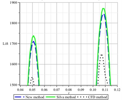
Fig. 6 shows the difference of the two first-kernels identified by using New Method and Silva Method respectively. Fig. 7 shows the prediction of aerodynamic forces by using CFD directly computational method and using convolution techniques to the same sinusoid input with the first-kernels of 2-ROM and 3-ROM respectively. It illustrates that the higher of the ROM is used the more accuracy the kernels are.

Fig. 6First kernels obtained in Silva Method and New Method

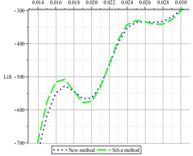
Fig. 7Lift predicted by using CFD method and convolution techniques respectively with first-kernels of 2-ROM and 3-ROM to the same sinusoid input

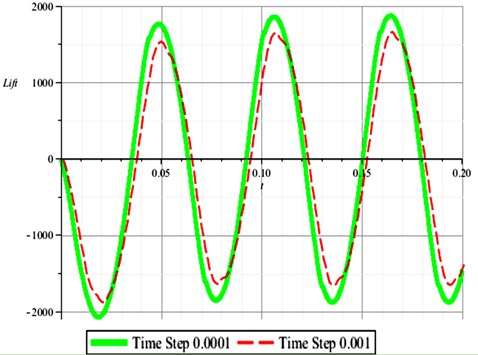
Note that the accuracy of the prediction of aerodynamic forces using CFD directly computational method is dependent on the choice of the time step. Fig. 8 shows the difference of the accuracy when executing CFD code with the step time 0.001 and 0.0001 respectively. The input is given by $u\left(t\right)=0.1\mathrm{s}\mathrm{i}\mathrm{n}\left(108.36t\right)$. However, it does not a matter to consider the selection of time step size in the view of identification which is merely concerned about data of inputs and outputs.

Fig. 8CFD Results based on time step 0.001, 0.0001

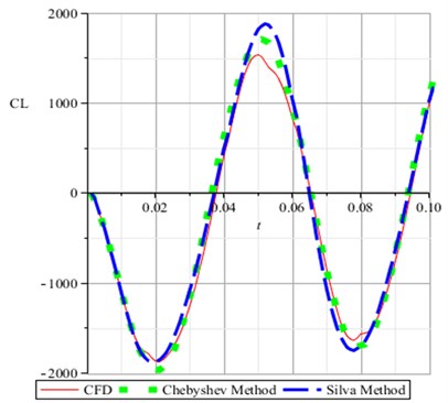
Using CFD method, impulse-response method (Silva method based on 2-ROM) and Chebyshev polynomials method (our new method based on 3-ROM), the response curves is given respectively in Fig. 9.

Fig. 9Response curves computed by CFD, Chebyshev method and Silva method respectively

6. Conclusions

In order to improve the accuracy of identification, the third-order ROM is first proposed to model the nonlinear and unsteady aerodynamic forces. The second example shows the kernels of third-order ROM are much more accurate than those of a second-order ROM.

In order to overcome the prohibitively expensive time-consumptions by executing CFD code to get the fully data for identification in an impulse- or step-response method, Chebyshev polynomials method is suggested and investigated in details. This method of identification is classified as a parameter method. Since only parts of the data are used for identification, the number of executing CFD code can be reduced at least one order of magnitude. That is extremely time-saving.