Abstract
A two-dimensional finite volume model is developed for the unsteady, and shallow water equations on arbitrary topography. The equations are discretized on quadrilateral control volumes in an unstructured arrangement. The HLLC Riemann approximate solver is used to compute the interface fluxes and the MUSCL-Hancock scheme with the surface gradient method is employed for second-order accuracy. This study presents a new method for translation of discretization technique from a structured grid description based on the traditional (, ) duplet to an unstructured grid arrangement based on a single index, and efficiency of proposed technique for unsplit finite volume method. In addition, a simple but robust well-balanced technique between fluxes and source terms is suggested. The model is validated by comparing the predictions with analytical solutions, experimental data and field data including the following cases: steady transcritical flow over a bump, dam-break flow in an adverse slope channel and the Malpasset dam-break in France.
1. Introduction
A sudden increase in discharge from dam or levee breaks can generate shock waves of discontinuous flow properties. Discharge discontinuity ultimately leads to water surface discontinuity. It is difficult to find exact solutions to these discontinuous flows through the linearization of non-linear equations. With the introduction of the total variation diminishing (TVD) method and an approximate Riemann solver, there has been an innovative advance in second or higher order accurate schemes that can be applied to analyzing discontinuous shock waves such as dam-break waves. However, the high resolution schemes face challenges such as an imbalance between fluxes and source terms in steady flows over an irregular bed. The imbalance is caused by the inaccurate discretization of source terms, such as the bed slope in shallow water equations. Accordingly, various numerical techniques for treating source terms in an effective way, so-called well-balanced schemes, which would make it possible to maintain the balance between fluxes and source terms under steady-state conditions, have been proposed.
Bermudez and Vázquez [1] introduced the C-property, which shows validity for conservation laws in still water by dividing the vector and scalar terms in the shallow water equations and discretizing the source terms by upwind schemes. LeVeque [2] proposed a quasi-steady wave algorithm that recomposes the fluxes by introducing an artificial discontinuity within each computational cell. However, this algorithm cannot provide accurate solutions for a steady transcritical flow with a shock. Zhou et al. [3] proposed a surface gradient method (SGM) for accurately treating source terms such as the bed slope. The method was extended to the SGMS [4], which is capable of treating bed topographies including a vertical step, and was validated by laboratory data with various bed slopes. Bradford and Sanders [5] introduced a new technique for handling numerical truncation errors induced by the pressure and bed slope terms in an arbitrary topography with moving lateral boundaries. Burfau et al. [6] solved the 1D and 2D unsteady shallow water equations using the cell-centered Roe finite volume scheme and an upwind discretization of the bed slope. Rogers et al. [7] proposed an algebraic technique using Roe’s approximate Riemann solver for keeping the balance between flux gradients and source terms. Valiani and Begnudelli [8] introduced the divergence form for bed slope source term (DFB) as a possible basis of any numerical integration method for the 1D or 2D SWE. Caleffi and Valiani [9] presented a new method called a finite volume well-balanced weighted essentially nonoscillatory (WENO) scheme to manage bed discontinuities. Pu et al. [10] proposed a surface gradient upwind method (SGUM) to combine the merit of SGM and depth gradient method (DGM) by including the source terms into the inviscid flux discretization.
This study develops a well-balanced finite volume model applicable to natural rivers using the unsplit method. The unsplit method considers the conserved variables in all directions of space simultaneously. Hence, this approach is very effective and flexible in dealing with unstructured meshes which are robust in generating computational domains with highly complex boundary shapes. To calculate the flux at the interfaces between the cells through the use of the unsplit method, information for both computational and neighboring cells should be known. To achieve this, this study introduces an efficient algorithm to automatically find neighboring cells of computational cells and to determine the order of the neighboring cells even in complex calculation domains composed of unstructured meshes. Also, this work proposes a simple technique to preserve a well-balanced solution in a dry bed and a new boundary-handling technique that can enable the effective application of an unsplit method.
The proposed model is validated through the comparison of numerical solutions and analytical solutions to steady transcritical flow over a bump. It is also applied to the dam-break flow in an adverse slope channel using laboratory data. Finally, the accuracy and reliability of the numerical model based on a Godunov-type scheme are verified with a natural topography through the simulation of the Malpasset dam-break by comparing simulated results, field surveyed data and experimental measurements.
2. Governing equations
The numerical model solves the two-dimensional shallow water equations as governing equations. The two-dimensional shallow water equations can be written in matrix form as:
where is the conserved variable vector, and are the fluxes in the and directions, respectively, represents a source term, and are the velocity in the and directions, respectively, is the water depth and and are the bed slope and friction slope terms, respectively.
3. Numerical model
3.1. Finite volume method
The governing equations are discretized based on the cell centered finite volume method. By integrating Eq. (1) over an arbitrary computational cell, the basic equation of finite volume method can be obtained as:
where is the boundary of the cell, is the outward unit vector that is normal to the boundary , and is the normal flux vector and can be determined by using the rotational invariance property [11]:
where is the angle between the outward unit vector and the -axis, represent the transformed conserved variables, is the transformed normal flux, and and are the transformation matrix and its reverse, respectively:
therefore, Eq. (3) can be discretized as [12]:
where is the area of an integration cell, is the number of cell interfaces, is the index of the cell interface, and is the width of each interface.
3.2. HLLC approximate Riemann solver
The HLL approximate Riemann solver [13] cannot take into account intermediate waves, such as shear waves or contact discontinuities [11]. To correct the defects of the HLL approach, Toro et al. [14] proposed a modified method called the HLLC scheme, in which C stands for Contact. The HLLC scheme provides results that satisfy the entropy condition [15]. If wave speeds are properly calculated and applied, the HLLC scheme can easily handle dry beds as well [16]. It also provides successful approximate solutions to practical applications [17].
Fig. 1Wave structure of the HLLC approximate Riemann problem
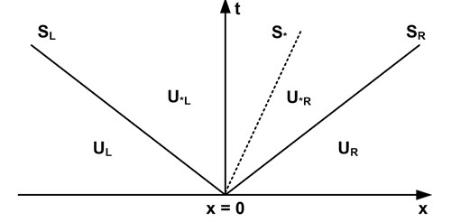
Fig. 1 shows the structure of waves assumed in the HLLC approximate Riemann solver. The conserved variable is divided into four parts according to wave speeds, and . If the conserved variables in each region have been determined, the HLLC numerical fluxes are evaluated from [11]:
where , , and and are the left and right Riemann states at each interface, respectively. and are the numerical fluxes in the left and right parts of the star region of the Riemann solution separated by a contact wave, respectively, and , and are the speeds of the left, contact and right waves, respectively.
To properly apply the HLLC approach to shallow water equations, it is important to calculate correct wave speeds , and [18]. In this study, a computational cell and a neighboring cell are set as the left and right hand sides of the Riemann interface for correctly calculating wave speeds using the unsplit method (Fig. 2(b)). At the same time, the wave speeds , and are estimated by taking into account the wet and dry bed conditions. The combinations of existing relations among wave speeds and are shown in Table 1.
Table 1Wave speeds for wet and dry beds
Wet bed | Dry bed | ||
Rarefaction wave | Shock wave | Computational cell () | Neighboring cell () |
In Table 1, , , and are the left and right initial values for a local Riemann problem. The contact wave speed , water depth and () are calculated from [11]:
3.3. Linear reconstruction of unsplit finite volume scheme
The MUSCL-Hancock scheme is a second-order extension of the Godunov upwind method. This scheme reconstructs conserved variables at the interface between cells prior to the calculation of fluxes for second-order accuracy in space and predicts fluxes at for second-order accuracy in time. To achieve second-order accuracy in space and time, the two-step MUSCL-Hancock method consisting of prediction and correction procedures is employed.
In the prediction step, the reconstruction of conserved variables is implemented at the interface between cells by using the data of both computational cells and neighboring cells. The simultaneous reconstruction of conserved variables at each interface is required to predict fluxes using the unsplit method. Thus, information about a computational cell and its neighboring cells, including cell numbers and primitive variables, must be known, and the order of the neighboring cells needs to be determined for two-dimensional calculations. To obtain the information necessary for calculation, the following algorithm is introduced in this study:
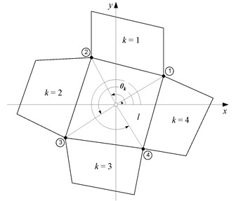
1) The angles produced by the centroid coordinate of a computational cell and the coordinates of nodes consisting of a computational cell are calculated using Eq. (11) for all cells in the computational domain:
2) As shown in Fig. 2(a), the index of nodes is determined in ascending order based on the angles calculated in the previous step.
3) Two nodes from the lowest number are read counter-clock wise for a computational cell. At the same time, the node numbers for the other cells, except the computational cell, are read in the same manner. The process is repeated to find the nodes matched with the two previously read nodes.
4) The cells with two shared nodes become the computational cell and one of its neighboring cells. The order of neighboring cells is determined in the order of angles produced between the centroid and the nodes of the computational cell.
The proposed algorithm can be easily applied without any limits to the configuration of cells, even in complex flow domains such as natural rivers.
Fig. 2Schematic diagram of topological relationships between cells a) The order of neighboring cells and b) Linear reconstruction at interface for unsplit scheme
a)
b)
The SGM [3] is coupled with the MUSCL-Hancock scheme so as to keep the balance between flux gradients and source terms. The SGM uses the water level instead of the water depth of depth gradient method (DGM) for reconstruction of conserved variables at interfaces in the prediction procedure. Accordingly, , which is the variation of , instead of the variation of is estimated as:
where is a computational cell and 1, 2, 3 and 4 represent the index of neighboring cells composing cell (Fig. 2(a)). To prevent numerical oscillations that may occur near discontinuities with the use of the second-order-accurate MUSCL-Hancock method, the TVD scheme, which limits the slopes of conserved variables to be reconstructed at the interface, is applied in this study. The Superbee limiter [11] is extended to the and directions for unsplit scheme application as Eq. (13):
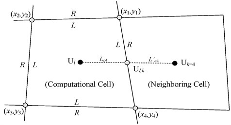
For linear reconstruction of flow variables at interface, the method which uses the distance between the center of a computational cell and midpoint of edges is employed (Fig. 2(b)). This technique is efficient to treat uniform or nor-uniform mesh since it can capture the correct behavior of linear function within a cell [13]. Therefore, for each interface between cells is extrapolated as:
where (1, 2, 3 and 4) is the distance from the center of cell to each midpoint of interface (Fig. 2(b)). To estimate the conserved variable needed to calculate the fluxes at the interfaces, and , both of which are conserved variables of momentum equation calculated in Eq. (14), and , which is the conserved variable of the continuity equation calculated in Eq. (15), are used [13]:
where , and refer to the water depth, water level and average bed elevation at interfaces between a computational cell () and neighboring cells (). Audusse et al. [20] suggested instead of Eq. (15) to preserve nonnegative water depth. However, this suggestion can cause imbalance between fluxes and sources terms in dry bed [21]. In this study, a simple technique propose to preserve nonnegative water depth and the well-balanced solutions in a dry bed application as Eq. (16):
where is the counterpart number of (e.g., 1, 3).
The prediction fluxes and are obtained by substituting the conserved variables at interfaces into Eq. (2). For second-order accuracy in time, a conserved variable in is computed as:
where is the area of the cell , is the computational time step, is the number of the neighboring cells of cell , and are the and components of the normal outward unit vector of the interface ( and is the width of the interface.
In the correction step, a conserved value at the time level is achieved by solving a series of Riemann problems at the interface based on data from the prediction step [3, 19]:
where the correction fluxes and in the and directions are computed using the HLLC approximate Riemann solver.
3.4. Treatment of source terms
In developing a numerical model to compute shallow water flows with an irregular bed topography, the numerical treatment of source terms largely affects the accuracy of the calculated results [17, 22-23]. The SGM is accurate and effective in treating source terms and can be easily coupled with the MUSCL-Hancock scheme [3]. Accordingly, this study improved the accuracy and stability of the developed model by combining the two schemes. The source terms consist of two parts, including the bed slope and the friction slope.
For the discretization of the bed slope terms, the application of the divergence theorem yields the rate of change of bottom elevation in the and directions of cell as follows [22]:
where subscripts 1, 2, 3 and 4 represent the index of nodes composing the computational cell, as shown in Fig. 2(b). The friction slopes in the and directions are estimated using Manning’s formula with the wide channel assumption [24]:
where is Manning coefficient, and the primitive variables , and are estimated using the average values over the computational cell .
3.5. Boundary conditions
Fig. 3Assignment of ghost cell numbers for boundary condition treatment
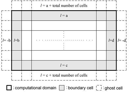
The finite volume method requires ghost cells for the treatment of the boundary condition. Fig. 3 depicts the computational domain and ghost cells. In this study, the numbers to be assigned to each ghost cell are determined using boundary cell numbers as shown in Fig. 3. This technique delivers an efficient treatment of complex topographies at the boundary. For general shallow water problems, two types of boundary conditions including the transmissive boundary condition and the reflective boundary condition are taken into account without considering the flow regime [11]. The Eq. (21) and (22) are used for a transmissive, and a reflective boundary condition, respectively:
where the subscripts and refer to the left hand side and right hand side of the Riemann states at the interface between boundary cells and ghost cells, respectively.
4. Applications
The developed model is applied to various test cases to assess the efficiency and accuracy of the algorithm proposed in this study. A steady flow over a bump and a dam-break flow in an adverse slope channel with flow conditions including steady transcritical flow, hydraulic jump, wet and dry fronts and reverse flow are considered, and the calculated results are compared with analytical solutions and experimental data. Additionally, the numerical model is applied to the Malpasset dam-break in France, and the application results are compared with field surveyed data and experimental data.
4.1. 1D Steady flow over a bump
If boundary conditions remain constant in a computational domain in which stationary flow is taken as the initial state, the flow will become steady-state despite the presence of a bed slope. However, nonphysical oscillations occur around the discontinuity of the bed slope if the source terms are not treated appropriately. Simulations investigating the convergence to a steady state are generally used to verify the balance between the flux gradients and source terms of a numerical model. In order to demonstrate convergence to a steady state, this study takes into account a channel proposed by Goutal and Manual [25]. The channel is frictionless and rectangular, 25 m in length and 1 m in width. The bed elevation is defined as:
According to the initial and boundary conditions, the steady flow over a bump can be subcritical or transcritical flow with or without a shock [25]. Of the three cases, subcritical flow and steady transcritical flow with a shock are selected for model verification, because the two cases are considered most challenging for a numerical model. We refer to Goutal and Maurel [25] for analytical solutions.
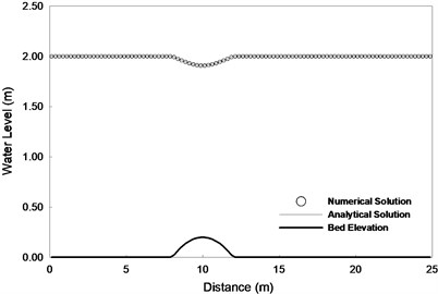
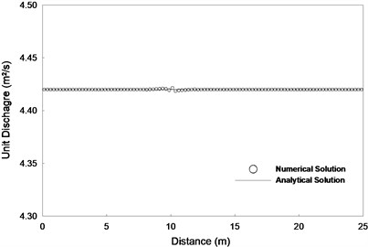
4.1.1. Subcritical flow
For the case of a subcritical flow, a constant discharge per unit width of 4.42 m2/s is specified at the upstream boundary and a fixed water level of 2 m is imposed at the downstream boundary. 2 m is also used as an initial value for the entire domain. For the computational domain, 100 cells with 0.25 m are composed. The Courant number is 0.9, and the simulation time is 360 seconds. Fig. 4 indicates that the model predictions are in good agreement with the analytical solutions for water level and discharge per unit width. Deviations between the simulation results and the analytical solutions are similar to other researchers’ results [3, 26-27].
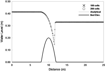
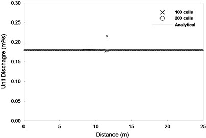
4.1.2. Transcritical flow with a shock
For the transcritical flow with a shock, a discharge per unit width of 0.18 m2/s is imposed at the upstream boundary and a water level of 0.33 m is fixed at the downstream boundary. The initial water level is 0.33 m throughout the entire computational domain, in which case the hydraulic jump occurs at the end of the bump.
Fig. 4Steady subcritical flow over a bump a) Water level and b) Discharge per unit width
a)
b)
To investigate accuracy dependence on cell size, simulations for 100 and 200 cells were carried out, respectively. Fig. 5 shows a comparison between the numerical predictions and analytical solutions for the water level and discharge per unit width estimated after 360 seconds. In both cases, numerical errors occur at the end of the bump. When the number of cells is 100, discharge near the point where the hydraulic jump occurs cannot meet steady-state conditions. On the other hand, when the number of cells is increased to 200, the numerical prediction is shown to have good agreement with analytical solutions. The maximum deviation between the discharge predictions and the analytical solutions is 15 % and 2 % for 100 and 200 cells, respectively. It is clearly shown that the error between the numerical solution and analytical solutions decreases as the number of cells increases.
Fig. 5Steady transcritical flow over a bump with a shock a) Water level and b) Discharge per unit width
a)
b)
The simulated results of the steady flow over a bump show close agreement with analytical solutions without spurious oscillations. This suggests that the unsplit method applied to the proposed algorithm in this study and the source-term treatment technique combined with the SGM maintains a numerical balance between fluxes and source terms.
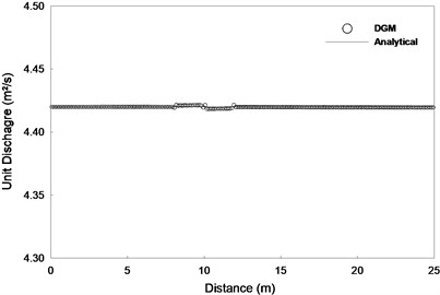
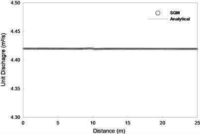
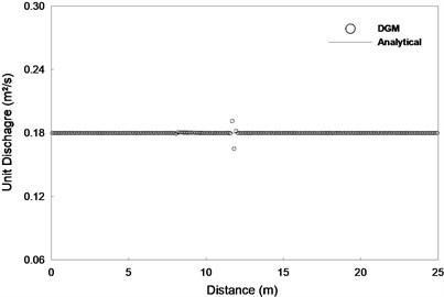
In order to assess the efficiency and accuracy of the source term treatment with the SGM in the developed model, a case with the DGM is employed for comparison. The SGM is the same as the DGM in procedure, except that it uses the water level instead of the water depth for the reconstruction of conserved variables at the interfaces between cells. The SGM and DGM are applied to the previous two test cases of steady flow over a bump, respectively. In those applications, 200 cells are used. Fig. 6 and 7 show a comparison of the unit discharge predictions of the SGM and DGM to subcritical flow and transcritical flow with a shock, respectively. In the comparison results, the numerical treatment of source terms using the DGM resulted in far larger numerical errors than that of source terms using SGM. This occurs because the DGM does not reflect the real variation of water depth [3]. As a result, the DGM cannot accurately reconstruct water depth at the interface. Thus, the incorrect reconstruction of water depth affected the entire calculation by causing an inaccurate estimation of fluxes at the interface. This demonstrates that the application of the SGM for the treatment of source terms can improve the accuracy and efficiency of the developed model.
Fig. 6Comparison of the DGM and SGM using the proposed model for steady subcritical flow over a bump a) DGM and b) SGM
a)
b)
Fig. 7Comparison of the DGM and SGM using the proposed mode for steady transcritical flow over a bump with a shock a) DGM and b) SGM
a)

b)
4.2. Dam-break flow in an adverse slope channel
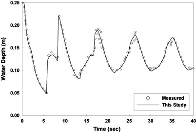
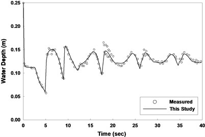
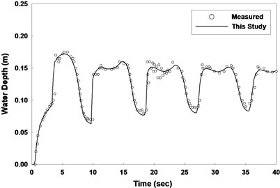
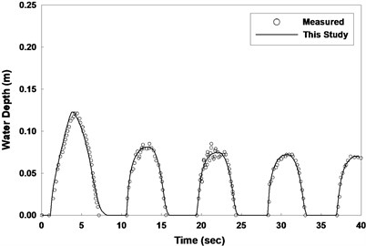
In this section, the accuracy of the proposed algorithm is verified through simulating dam-break experiments designed by Aureli et al. [28]. Laboratory experiments set up with different upstream depths and adverse slopes were intended to induce shock origination and propagation, a reverse flow and wetting and drying conditions. As shown in Fig. 8, the experimental domain was composed of a rectangular reservoir and a channel with an adverse slope connected to it. The length and width of this channel were set at 7 m and 1 m, respectively. To apply the numerical model, a computational domain consisting of 140 cells with 0.05 m and 1.0 m was composed. The Manning roughness coefficient is set to 0.010 m-1/3s, and the reservoir has an initial water depth of 0.25 m. The initial water depth downstream of the dam is zero for the dry bed test, and the total simulation time is set to 40 seconds. The side walls and upstream region of the channel have closed boundary conditions, and the downstream end has transmissive boundary conditions. Under these same conditions, Aureli et al. [28] and Tseng [29] validated a numerical model using the TVD-Maccormack scheme and the flux-limited TVD scheme, respectively. Fig. 8 shows the experimental configurations and simulation conditions. The bed topography is defined as:
Fig. 8Schematic view of the dam-break experiment in an adverse slope channel
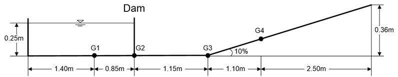
Fig. 9 shows a comparison of the calculated water depth and measured water depth at four different points. The simulated results for predicting the propagation time of the forward and reverse waves, wet/dry fronts and water depth are in close agreement with the observed values. From these simulated results, it can be demonstrated that a new method for a linear reconstruction of conserved variables in effectively applying an unsplit scheme and a simple technique to preserve balance between fluxed and source terms in a dry bed can handle reverse flow and wetting and drying beds very well.
Fig. 9Dam-break flow in an adverse slope channel: comparison of water depths at a) G1, b) G2, c) G3 and d) G4
a)
b)
c)
d)
4.3. Malpasset dam-break flow
To verify the applicability of the developed model to a natural river with an irregular bed elevation and dry terrain, it is applied to the Malpasset dam-break simulation. The dam was located in the valley of the Reyran River about 12 km upstream of the Frejus city in France and was constructed to provide irrigation and drinking water for that city in 1954. It was an arch dam with a maximum height of 66.5 m, a crest length of 223 m and a storage capacity of 55×106 m3. It collapsed due to a sudden rise of water level in the reservoir resulting from exceptional rainfall on December 2, 1959, and the resulting flood waves were propagated along the Reyran valley to Frejus, leaving 421 casualties [30]. This dam-break case was simulated by other researchers [30-33] to verify their numerical model.
The high water marks of flood waves resulting from the dam-break were surveyed by the police along the left and right banks of the Reyran River. Fig. 10 shows the surveyed points, including P1-P17. In 1964, a laboratory experiment on the Malpasset dam-break was conducted using a physical model scaled at 1:400, made by LNH-EDF. In the experiment, the arrival time of the flood wave and the maximum free surface elevations were measured in S6-S14 gauges as shown in Fig. 10 [32]. These data are used to validate the numerical model in this study. The boundary condition for the upstream region is an imposed reflective boundary condition without any inflow into the reservoir because it was very small in comparison to the discharge resulting from the dam-break [30]. The downstream boundary conditions are set as a free flow which flood waves run into the sea. For the initial conditions, the water level of the reservoir is imposed at 100 m, and the downstream region of the dam is considered as a dry bed. The 13,550 quadrilateral meshes composing the computational domain are used and Manning coefficient is specified at 0.033 m-1/3s for the entire area.
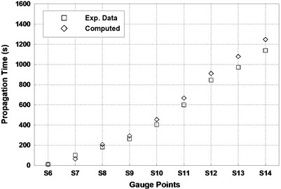
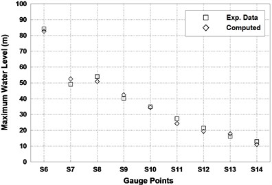
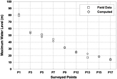
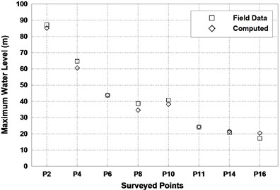
In Fig. 11, the predicted arrival time of the flood front and the maximum water surface elevation are compared with the measurements of the physical model. Fig. 12 shows a comparison of the calculated maximum water surface elevation with field data surveyed in the left and right banks. The predictions in the proposed model demonstrate relatively good agreement with the field and experimental data. However, there are small discrepancies between the simulation results and high water marks at surveyed points, P4, P5, P7, P8, P13 and P16. It should be noted that, in the simulation, bottom elevation data digitized from maps dating back to 1931 are used [30]. However, the field data were collected after the dam-break, which was accompanied by abrupt changes in topography. This may be the reason for differences between the numerical results and the high water marks.
Fig. 10Topography and locations of field surveyed points (P1-P17) and gauges at physical model (S6-S14)
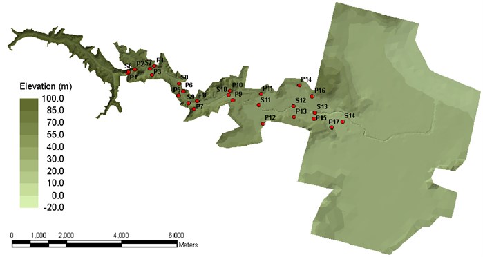
Fig. 11Comparison between predicted results and experimental data a) Propagation time at gauges, b) Maximum water level at gauges
a)
b)
Fig. 12Comparison between predicted results and field data a) Maximum water level at right banks, b) Maximum water level at left banks
a)
b)
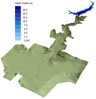
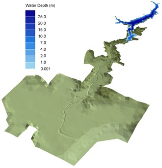
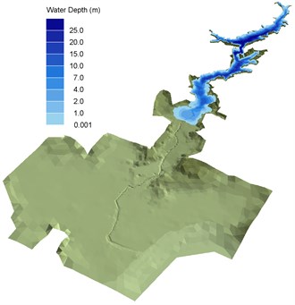
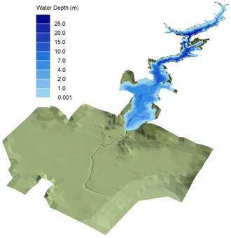
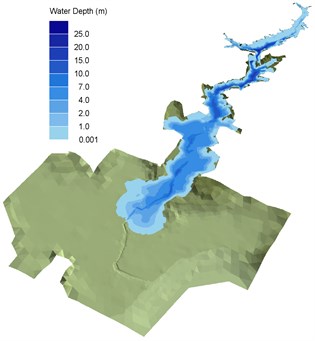
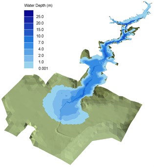
Fig. 13 illustrates the three-dimensional flood inundation extent and water depth distributions at 0, 3, 12, 21, 30 and 35 minutes after the dam-break. As shown in Fig. 13, the main channel in the center of the river valley is included in the topography and flood waves due to dam-failure are rapidly propagated along the steep and narrow valley, starting at the dam.
Fig. 133D inundation water depth and extent at a) 0, b) 3, c) 12, d) 21, e) 30 and f) 35 min
a)
b)
c)
d)
e)
f)
However, as the flood waves travel downstream, where the floodplain becomes wider, they are propagated more slowly and the water depth decrease. Additionally, the wave front is also propagated over a wider area. The water level, which is initially set to 100 m in the reservoir, dramatically drops for 35 minutes after the dam-break. Fig. 13 shows that the main characteristics of the flood resulting from the Malpasset dam-break can be well reproduced by the proposed model. It also reveals that the techniques presented in this study can be simply and efficiently applied to irregular topographies such as natural channels.
5. Conclusion
This study developed a well-balanced finite volume model that can be applied to irregular boundaries and complex bed topographies. The proposed model is based on the conservative form of the two-dimensional shallow water equations, and the HLLC approximate Riemann solver with MUSCL-Hancock scheme solves the equations by applying the unsplit method to achieve geometrical flexibility. An algorithm for finding neighboring cells to a computational cell for the efficient application of the unsplit method and a new scheme for handling ghost cells for the treatment of complex boundaries are proposed. In addition, a simple and robust technique to preserve nonnegative water depth and well-balanced solutions in a dry bed is suggested. The proposed model is validated through the comparison of predictions with analytical solutions, experimental data and field data. In this study, three test cases are considered. One is a steady flow over a bump, another is dam-break flow with an adverse slope and the last one is the Malpasset dam-break in France. Simulation results for the first two cases show that a balance between the flux gradient and source terms can be reached with the developed model. In addition, the proposed model gives accurate solutions to complex flows, including the interactions of multiple flows, reverse flow, dry/wet shock fronts and hydraulic jumps. In the Malpasset dam-break simulation, the developed model is capable of providing accurate predictions for the arrival time and the maximum water surface elevation of floods occurring in natural rivers. From the reasonable results of several test cases chosen for a numerical verification, it is demonstrated that the proposed model can provide high accuracy, flexibility and efficiency in handling various types of shallow water flows with arbitrary topography.
References
-
Bermudez A., Vázquez M. E. Upwind method for hyperbolic conservation laws with source terms. Computers & Fluids, Vol. 23, Issue 8, 1994, p. 1049-1071.
-
LeVeque R. J. Balancing source terms and flux gradients in high-resolution Godunov methods: the quasi-steady wave-propogation algorithm. Journal of Computational Physics, Vol. 146, Issue 1, 1998, p. 346-365.
-
Zhou J. G., Causon D. M., Mingham C. G., Ingram D. M. The surface gradient method for the treatment of source terms in the shallow-water equations. Journal of Computational Physics, Vol. 168, Issue 1, 2001, p. 1-25.
-
Zhou J. G., Causon D. M., Ingram D. M., Mingham C. G. Numerical solutions of the shallow water equations with discontinuous bed topography. International Journal for Numerical Methods in Fluids, Vol. 38, Issue 8, 2002, p. 769-788.
-
Bradford S. F., Sanders B. F. Finite-volume model for shallow-water flooding of arbitrary topography. Journal of Hydraulic Engineering, Vol. 128, Issue 3, 2002, p. 289-298.
-
Brufau P., Vázquez-Cendón M. E., Garcia-Navarro P. A. Numerical model for the flooding and drying of irregular domains. International Journal for Numerical Methods in Fluids, Vol. 39, Issue 3, 2002, p. 247-275.
-
Rogers B. D., Borthwick A. G. L., Taylor P. H. Mathematical balancing of flux gradient and source terms prior to using Roe’s approximate Riemann solver. Journal of Computational Physics, Vol. 192, Issue 2, 2003, p. 422-451.
-
Valiani A., Begnudelli L. Divergence form for bed slope source term in shallow water equations. Journal of Hydraulic Engineering, Vol. 132, Issue 7, 2006, p. 652-665.
-
Caleffi V., Valiani A. Well-balanced bottom discontinuities treatment for high-order shallow water equations WENO scheme. Journal of Engineering Mechanics, Vol. 135, Issue 7, 2009, p. 684-696.
-
Pu J. H., Cheng N. S., Tan S. K., Shao S. Source term treatment of SWEs using surface gradient upwind method. Journal of Hydraulic Research, Vol. 50, Issue 2, 2012, p. 145-153.
-
Toro E. F. Shock-capturing methods for free-surface shallow flows. John Wiley & Sons, New York, 2001.
-
Zhao D. H., Shen H. W., Tabios G. Q., Lai J. S, Tan W. Y. Finite-volume two-dimensional unsteady-flow model for river basins. Journal of Hydraulic Engineering, Vol. 120, Issue 7, 1996, p. 863-883.
-
Harten A., Lax P. D., Van Leer B. On upstream differencing and Godunov-type schemes for hyperbolic conservation laws. Journal of Computational Physics, Vol. 25, Issue 1, 1983, p. 35-61.
-
Toro E. F., Spruce M., Speares W. Restoration of the contact surface in the HLL Riemann Solver. Shock Waves, Vol. 4, Issue 1, 1994, p. 25-34.
-
LeVeque R. J. Finite volume methods for hyperbolic problems. Cambridge University Press, Cambridge, 2002.
-
Fraccarollo L., Toro E. F. Experimental and numerical assessment of the shallow water model for two-dimensional dam-break type problems. Journal of Hydraulic Research, Vol. 33, Issue 6, 1995, p. 843-864.
-
Zia A., Banihashemi M. A. Simple efficient algorithm (SEA) for shallow flows with shock wave on dry and irregular beds. International Journal for Numerical Methods in Fluids, Vol. 56, Issue 11, 2008, p. 2021-2043.
-
Liang Q., Borthwick A. G. L., Stelling G. Simulation of dam- and dyke-break hydrodynamics on dynamically adaptive quadtree grids. International Journal for Numerical Methods in Fluids, Vol. 46, Issue 2, 2004, p. 127-162.
-
Soares-Frazão S., Guinot V. An eigenvector-based linear reconstruction scheme for the shallow-water equation on two-dimensional unstructured mesh. International Journal for Numerical Methods in Fluids, Vol. 53, Issue 1, 2007, p. 23-55.
-
Audusse E., Bouchut F., Bristeau M. O., Klein R., Perthame B. A fast and stable well-balanced scheme with hydrostatic reconstruction for shallow water flows. SIAM Journal on Scientific Computing, Vol. 25, Issue 6, 2004, p. 2050-2065.
-
Liang Q. Flood simulation using a well-balanced shallow flow model. Journal of Hydraulic Engineering, Vol. 136, Issue 9, 2010, p. 669-675.
-
Guo W. D., Lai J. S., Lin G. F. Finite-volume multi-stage schemes for shallow-water flow simulations. International Journal for Numerical Methods in Fluids, Vol. 57, Issue 2, 2008, p. 177-204.
-
Aliparast M. Two-dimensional finite volume method for dam-break flow simulation. International Journal of Sediment Research, Vol. 24, Issue 1, 2009, p. 99-107.
-
Erduran K. S., Kutija V., Hewett C. J. M. Performance of finite volume solutions to the shallow water equations with shock-capturing schemes. International Journal for Numerical Methods in Fluids, Vol. 40, Issue 10, 2002, p. 1237-1273.
-
Goutal N., Maurel F. Proceedings of the 2nd workshop on dam-break wave simulation. Technical report HE-43/97/016, EDF-DER, Paris, 1997.
-
Vázquez-Cendón M. E. Improved treatment of source terms in upwind schemes for the shallow water equations in channels with irregular geometry. Journal of Computational Physics, Vol. 148, Issue 2, 1999, p. 497-526.
-
Ma D. J., Sun D. J., Yin X. Y. Solution of the 2-D shallow water equations with source terms in surface elevation splitting form. International Journal for Numerical Methods in Fluids, Vol. 55, Issue 5, 2007, p. 431-454.
-
Aureli F., Mignosa P., Tomirotti M. Numerical simulation and experimental verification of Dam-Break flows with shocks. Journal of Hydraulic Research, Vol. 38, Issue 3, 2000, p. 197-206.
-
Tseng M. H. Improved treatment of source terms in TVD scheme for shallow water equations. Advances in Water Resources, Vol. 27, Issue 6, 2004, p. 617-629.
-
Valiani A., Caleffi V., Zanni A. Case study: malpasset dam-break simulation using a two-dimensional finite volume method. Journal of Hydraulic Engineering, Vol. 128, Issue 5, 2002, p. 460-472.
-
Brufau P., García-Navarro P., Vázquez-Cendón M. E. Zero mass error using unsteady wetting – drying conditions in shallow flows over dry irregular topography. International Journal for Numerical Methods in Fluids, Vol. 45, Issue 10, 2004, p. 1047-1082.
-
Liang D., Lin B., Falconer R. A boundary-fitted numerical model for flood routing with shock-capturing capability. Journal of Hydrology, Vol. 332, Issue 3-4, 2007, p. 477-486.
-
Kim B., Sanders B. F., Schubert J. E., Famiglietti J. S. Mesh type tradeoffs in 2D hydrodynamic modeling of flooding with a Godunov-based flow solver. Advances in Water Resources, Vol. 68, 2014, p. 42-61.
About this article

This research was supported by Yeungnam University research grant in 2014 and a Development of Flooding Disaster Mitigation Standard Model and Advanced Management Technology [NEMA-NH-2014-04] from the Natural Hazard Mitigation Research Group, National Emergency Management Agency of Korea.
