Chaotic information-geometric support vector machine and its application to fault diagnosis of hydraulic pumps

Wang, Zhipeng; Lu, Chen; Wang, Zili

Journal of Vibroengineering

Browse Journal

Submit article

Published: 31 March 2014

Check for updates

Chaotic information-geometric support vector machine and its application to fault diagnosis of hydraulic pumps

Zhipeng Wang¹

Chen Lu²

Zili Wang³

^{1, 2, 3}School of Reliability and Systems Engineering, Beihang University, Beijing, 100191, China

^{1, 2, 3}Science and Technology on Reliability and Environmental Engineering Laboratory, Beijing, 100191, China

Corresponding Author:

Chen Lu

Cite the article Download PDF

Downloads 1098

Abstract

Fault diagnosis of rotating machineries is becoming important because of the complexity of modern industrial systems and the increasing demands for quality, cost efficiency, reliability, and safety. In this study, an information-geometric support vector machine used in conjunction with chaos theory (chaotic IG-SVM) is presented and applied to practical fault diagnosis of hydraulic pumps, which are critical components of aircraft. First, the phase-space reconstruction of chaos theory is used to determine the dimensions of input vectors for IG-SVM, which uses information geometry to modify SVM and improves performance in a data-dependent manner without prior knowledge or manual intervention. Chaotic IG-SVM is trained by using the dataset from the normal state without fault, and a residual error generator is then designed to detect failures based on the trained chaotic IG-SVM. Failures can be diagnosed by analyzing residual error. Chaotic IG-SVM can then be used for fault clustering by analyzing residual error. Finally, two case studies are presented, and the performance and effectiveness of the proposed method are validated.

1. Introduction

To reduce costs and shorten repair time, technologies for machine maintenance, diagnostics, and prognostics have received significant attention. Fault diagnosis is an essential prerequisite for the further development of automatic supervision. Real-time condition monitoring that can detect, classify, and predict impending faults is critical to reduce operating and maintenance costs [1]. Moreover, condition monitoring is important to increase machinery availability and improve manufacturing process productivity and reliability [2].

Hydraulic pumps are the power sources of hydraulic systems in aircraft. The performance of these pumps directly affects the stability of the hydraulic system and even that of the entire system. Statistical data show that hydraulic pumps have higher fault probability than other mechanical systems. Therefore, diagnosing pump health in real time is an important factor to increase the reliability and performance of hydraulic systems. If a fault-detection scheme that provides early warning of component failures can be developed, then repairs or replacements can be carried out at the earliest or most convenient time with minimum productivity loss [3]. However, hydraulic pumps are complex and have a high degree of coupling [4]. Considering complexity and severe working conditions, a data-driven fault-detection method is typically applied to online fault diagnosis. Many data-driven methods have been proposed, such as wavelet decomposition [5], artificial neural networks (ANNs) [6, 7], fuzzy logic, kernel principal component analysis [8], and D-S evidence theory [9].

Given the universal presence of chaotic phenomena and the intrinsic characteristics and complex operating conditions of hydraulic systems, strong nonlinearity and chaotic features can clearly be observed in the vibration signals of hydraulic pumps [7]. Therefore, chaos theory is valuable for the fault diagnosis of hydraulic pumps [10].

A support vector machine (SVM), as a data-driven method, has been widely applied. Compared with ANNs, SVM overcomes numerous defects such as overfitting and local convergence. In addition, SVM has advantages over ANNs in terms of robustness and in preventing the curse of dimensionality. SVM has been applied to many fields, such as in pattern recognition and fault diagnosis [1].

Despite its excellent applicability, the performance of SVM largely depends on the kernel [11, 12]. Kernel functions are mostly chosen based on experience. However, unsuitably chosen kernel functions may significantly impair performance [13]. No systematic approach for choosing appropriate kernel functions has yet been introduced [14]. Choosing a kernel corresponds to a smoothness assumption of the discriminant function of the classifier. When we have prior knowledge, we can use it to choose a kernel [15, 16]. In practice, however, prior knowledge is typically unavailable. Therefore, the kernel should be optimized in a data-dependent manner. An information-geometric method is employed in the present study. Based on the structure of the Riemannian geometry induced in the input space by the kernel, SVM can be modified in a data-dependent manner, and information-geometric SVM (IG-SVM) can be obtained.

This paper is divided into three sections. Section 2 describes chaos theory on phase-space reconstruction, proposes a new IG-SVM for chaotic time-series prediction, and describes the designed residual error generator. Sections 3 and 4 present several case studies, including the simulation results of a one-step iterative prediction and the experimental results of fault detection for a hydraulic pump. The feasibility and efficiency of the method are validated via a plunger pump test bed.

2. Methodology

2.1. Phase-space reconstruction of a chaotic time series

Phase-space reconstruction theory regards a 1D chaotic time series as the compressed information of high-dimensional space. The Takens embedding theorem [17] suggests that a dependable phase-space reconstruction of a dynamic system can be obtained if:

1

m \geq 2 D + 1,

where $m$ is the system embedding dimension, and $D$ is the dimension of the system attractor. To obtain a correct system embedding dimension, $D$ should be estimated starting from the time series.

The correlation dimension, as defined by Grassberger and Procaccia, is a popular definition because of its calculation simplicity [18]. The correlation integral $C_{m} (r)$ is defined as:

2

C_{m} (r) = \frac{2}{N (N - 1)} \sum_{i = 1}^{N} \sum_{j = i + 1}^{N} H (r - |X_{i} - X_{j}|),

where $H$ is the Heaviside function, $m$ is the embedding dimension, and $N$ is the number of vectors in the reconstructed phase space. If $r$ is sufficiently small and $N$ is sufficiently large, then the correlation dimension $D$ is equal to:

3

D = \underset{r \to 0}{l i m} \frac{l n (C_{m} (r))}{l n (r)} .

The algorithm plots a cluster of $ln {(C}_{m} (r)) - ln (r)$ curves by increasing $m$ until the slope of the linear part of the curve is nearly constant. The correlation dimension D can then be estimated.

2.2. Modified SVM that uses information geometry

The SVM proposed by Vapnik [16] aims to minimize an upper bound of the generalization error by maximizing the margin between the separating hyperplane and the data. Consider a pattern classifier that uses a hyperplane to separate two classes of patterns based on given examples $= \{(x_{1}, y_{1}), \dots, (x_{i}, y_{i})\}$ , where $x$ is a vector in the input space $S = R^{d}$ , $y \in {- 1,1}$ is a class label, and $i =$ 1,…, $l$ . A nonlinear SVM maps the input data $x$ onto a high-dimensional feature space $F = R^{n}$ ( $N$ may be infinite) via nonlinear mapping $ϕ (x)$ . Then, SVM searches for a linear discriminant function, that is:

4

f (x) = w ϕ (x) + b .

The basic concepts of SVM theory are comprehensively explained in [13]. Once the correlation dimension $D$ is obtained by using the Grassberger-Procaccia (GP) algorithm, the number of input nodes in SVM can be determined as:

5

I n = [2 D + 1] .

To modify the SVM kernel by using information geometry, the geometrical structure induced in the input space by a kernel should be analyzed as follows [19].

Mapping $ϕ (x)$ defines an embedding of $S$ into $F$ as a curved submanifold. When $F$ is a Euclidean or Hilbert space, a Riemannian metric is induced in space $S$ , wherein the length of a small line element $d x$ in $S$ is defined by the length in larger space $F$ .

$z$ denotes the mapped pattern of $x$ in the feature space, i.e., $z = ϕ (x)$ . A small vector $d x$ is mapped onto:

6

d z = \nabla ϕ (x) d x = \sum_{i} \frac{\partial}{\partial x_{i}} ϕ (x) d x_{i},

where:

7

\nabla ϕ (x) = \frac{\partial}{\partial x_{i}} ϕ (x) .

The squared length of $d z = d z_{α}$ is written in quadratic form as:

8

|d z| = \sum_{α} {(d z_{α})}^{2} = \sum_{i, j} g_{i j} (x) d x_{i} d x_{j},

where:

9

g_{i j} (x) = (\frac{\partial}{\partial x_{i}} ϕ (x)) ∙ (\frac{\partial}{\partial x_{j}} ϕ (x)) .

The dot denotes the summation over index $α$ of $ϕ .$ The $n \times n$ positive-definite matrix $G (x) = g_{i j} (x)$ is the Riemannian metric tensor induced in $S$ . This matrix shows that the metric is directly derived from the kernel.

The following is a theorem presented in [19]:

10

g_{i j} (x) = \frac{\partial}{\partial x_{i}} \frac{\partial}{\partial x_{i}^{'}} {K (x, x^{'})|}_{x^{'} = x},

the proof of which is:

11

\frac{\partial}{\partial x_{i}} \frac{\partial}{\partial x_{i}^{'}} K (x, x^{'}) = \nabla ϕ (x) ∙ \nabla ϕ (x^{'}) .

This proof verifies Eq. (10) [11].

Based on the preceding analysis, forecasting precision in regression problems can be improved if a special nonlinear map $ϕ$ is constructed, such that $g_{i j} (x)$ is reduced around the neighboring areas of the hyperplane $|y - f (x) - b| = ξ$ , which is contrary to the method used by Amari [11] in classification problems. This concept can be implemented by a conformal transformation of the kernel, that is:

12

\tilde{K} (x, x^{'}) = c (x) c (x^{'}) K (x, x^{'}),

with a properly positive scalar function $c (x)$ . $\tilde{K} (x, x^{'})$ is called the conformal transformation of a kernel by factor $c (x)$ . The nonlinear mapping $ϕ (x)$ can be regarded as being modified to $\tilde{ϕ} (x) = c (x) ϕ (x)$ , thus satisfying the Mercer positivity condition.

The metric ${\tilde{g}}_{i j} (x)$ can be obtained as follows:

13

{\tilde{g}}_{i j} (x) = c {(x)}^{2} g_{i j} (x) + c_{i} (x) c_{j} (x) + 2 c_{i} (x) c (x) K (x, x),

where $c_{i} (x) = \partial c (x) / \partial x_{i}$ and ${K_{i} (x, x) = \partial K (x, x^{'}) / \partial x_{i}|}_{x^{'} = x}$ . The last term is zero for the Gaussian radial basis function kernel.

Therefore, if we choose function $c (x)$ , such that its value is large when $x$ is close to the boundary and small otherwise, then we can enlarge the spatial resolution around the boundary [11].

Considering the preceding analysis, $c (x)$ can be chosen as:

14

c (x) = \frac{1}{m} \sum_{i = 1}^{m} e x p (- \frac{{‖x - o_{i}‖}^{2}}{τ^{2}}),

where parameters $m$ , $o_{i}$ , and $τ$ are the number of partitioning points, the center of the $i$ th partition, and the width of the $i$ th partition, respectively. Outside the circles, the value of $c (x)$ and its derivative are extremely small [15]. Therefore, this function satisfies the aforementioned requirement and can be used to modify SVM in a data-dependent manner.

2.3. Residual error generator

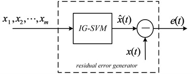
A residual error generator can be designed for fault diagnosis based on the IG-SVM prediction process. The structure is shown in Fig. 1.

In Fig. 1, $x (t)$ is the time series that can be observed in the actual system, IG-SVM is the residual error generator trained by the data from the normal state, $\hat{x} (t)$ is the one-step prediction value of IG-SVM, and $e (t)$ is the output of the residual error generator.

The diagnostic decision is obtained based on the following rule:

r_{e v a l} > J_{t h}

r_{e v a l} \leq J_{t h}

where $r_{e v a l}$ is the mean absolute value of the residual error signal, and $J_{t h}$ is the threshold that can be determined by experience.

Fig. 1Structure of the residual error generator based on IG-SVM

3. Simulation results

To verify the proposed method, the simulation result of Lorenz attractor data is provided. Eq. (15) is employed to generate Lorenz time-series data:

15

\{\begin{array}{l} d x = - σ x + σ y, \\ d y = - x z + r z - y, \\ d z = x y - b z, \end{array}

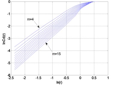
where $σ =$ 10, $r =$ 28, and $b =$ 8/3. A total of 1000 points of $X$ -component Lorenz time series were used for the following prediction. According to the GP algorithm, the embedding dimension can be determined, $m =$ 6.

Fig. 2Plot of lnCm(r)-ln(r) of the Lorenz time series

As a whole, 200 points were divided into two groups (i.e., the training and testing datasets). The first 100 samples were used for SVM training. The next 100 samples were employed to test the prediction accuracy between SVM and IG-SVM.

Fig. 3The one-step iterative predicted result of the Lorenz time series

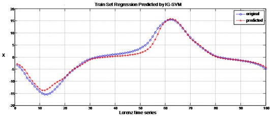
Fig. 4Comparison of APE between SVM and IG-SVM

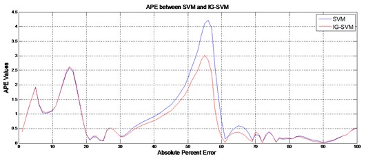
The number of input nodes of SVM was 6, which was obtained by estimating the minimum embedding dimension. Fig. 3 shows the one-step iterative predicted result for the last 100 points of the Lorenz time series by IG-SVM. Fig. 4 shows a comparison of the absolute percent error (APE) of the Lorenz time series between SVM and IG-SVM. Compared with SVM, IG-SVM exhibits better performance in iterative prediction in terms of convergence and stability.

4. Experimental results

In this section, a test rig of an SCY hydraulic plunger pump was evaluated and analyzed to verify the proposed method. In the experiment, two common types of faults in the plunger pump were set: (1) a wear fault between the swash plate and the slipper and (2) a wear fault of the valve plate. Under three different states, including the normal state, a vibration signal was acquired from the end face of the plunger pump at a stabilized motor speed of 528 r/min and a sampling rate of 1000 Hz.

Table 1 shows the corresponding maximum Lyapunov exponents ( $λ_{m a x}$ ) of the three datasets. Given that all $λ_{m a x}$ values are positive, the experimental data can be regarded as a chaotic time series.

Table 1Lyapunov exponents of the datasets of the hydraulic pump

Data	State	$λ_{m a x}$
Data 1	Normal condition	0.0508
Data 2	Wear fault between the swash plate and the slipper	0.0744
Data 3	Wear fault of the valve plate	0.0435

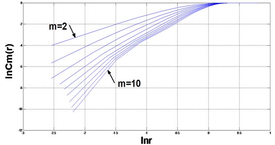
Following the GP method, a cluster of $ln C_{m} (r) - ln (r)$ curves for Data 1 is plotted with the increase in embedding dimension $m$ (Fig. 5). The correlation dimension can be determined correspondingly, $D =$ 2.2346. According to (1), $m =$ 6.

Fig. 5Plot of lnCm(r)-ln(r) of data from the hydraulic pump under the normal state

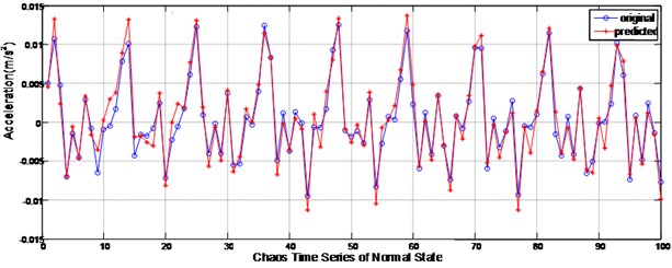
In this case, 200 points of the time-series data from the normal state were used. The first 100 samples were employed to train SVMs, whereas the last 100 samples were used to test and determine the threshold of fault diagnosis. After training and testing, a prediction model of the normal state is determined. Fig. 6 shows the result of using the one-step, iterative, prediction-based IG-SVM.

Fig. 6The one-step iterative predicted result of data from the normal state

4.1. Residual error of the normal state

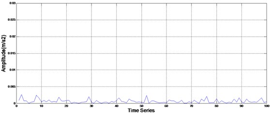
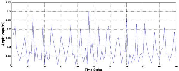
The residual error of the normal state data can be obtained by using the residual error generator. As mentioned earlier, $r_{e v a l}$ , which is the mean absolute value of the residual error, is used for fault clustering. Fig. 7 shows the absolute value of the residual error of the normal state.

Fig. 7Absolute value of the residual error of the normal state

4.2. Residual error of the wear fault between the swash plate and the slipper

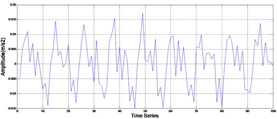
In this case, 100 points of the time-series data from the vibration signal with a wear fault between the swash plate and the slipper were used via the residual error generator. Fig. 8 shows the absolute value of the residual error of the wear fault between the swash plate and the slipper.

Fig. 8Absolute value of the residual error of the wear fault between the swash plate and the slipper

4.3. Residual error of the wear fault of the valve plate

In this case, 100 points of the time-series data from the vibration signal of the hydraulic pump with a wear fault of the valve plate were used for fault detection. Fig. 9 shows the absolute value of the residual error of the wear fault of the valve plate.

Fig. 9Absolute value of the residual error of the wear fault of the valve plate

4.4. Fault clustering

In this study, two groups of normal data and eight groups of faulty data in different fault types were acquired via the test rig. The residual error series was calculated by using the residual error generator based on IG-SVM. The absolute values of the residual error series are shown in Table 2.

Table 2 indicates that different types of data can be distinguished clearly by the absolute value $r_{e v a l}$ of the residual error. The threshold of normal data is typically set to a standard of that is three to five times higher than the means of the absolute values for normal data. In the present case, the threshold of Data1 is $J_{t h} =$ 27.23e-004. All $r_{e v a l}$ values of faulty data are greater than the $J_{t h}$ of Data 1, and faults can be detected successfully.

In addition, the $r_{e v a l}$ of Data 2 ranges from 65 to 75, whereas that of Data 3 ranges from 85 to 95. Therefore, the types of faults can also be isolated. The results show a 100 % success rate in correctly detecting and isolating hydraulic pump faults.

Table 2Absolute values of the residual error series

No.	Data 1		Data 2				Data 3
State	Normal (e-004)		Wear fault between the swash plate and the slipper (e-004)				Wear fault of the valve plate (e-004)
Data	1-1	1-2	2-1	2-2	2-3	2-4	3-1	3-2	3-3	3-4
$r_{e v a l}$	5.36	5.53	73.523	72.39	68.11	66.95	92.91	93.13	89.11	87.27
Mean ( $r_{e v a l}$ )	5.45		70.24				90.60
Threshold $J_{t j}$	27.23		65 to 75				85 to 95

5. Conclusion

Fault diagnostics is the primary technique used for condition-based predictive maintenance. This approach can reduce costs and shorten repair time. The strong nonlinearity and chaotic features of the vibration signals of hydraulic pumps result in difficulties in fault diagnosis. This study presents a fault diagnosis method based on chaotic IG-SVM, which improves the performance of SVM in a data-dependent manner. The simulation results show that IG-SVM, when used in conjunction with phase-space reconstruction, exhibits better capability and reliability in predicting a chaotic time series, as well as high-performance convergence ability and prediction precision in the short-term prediction of a chaotic time series. The experimental results show that the IG-SVM model demonstrates a strong ability to approximate the output and state of a normal system, which is useful in fault detection. Additional works are necessary to validate the proposed method further for wider applications. Moreover, determining thresholds automatically is another issue that should be addressed.

References

Xiaoming H. Study on fault diagnosis of hydraulic pump based on sphere-structured support vector machines. 2nd International Conference on Consumer Electronics, Communications and Networks, 2012, p. 2894-2896.

Search CrossRef
Gertler J. J. Survey of model-based failure detection and isolation in complex plants. Control Systems Magazine, Vol. 8, 1988, p. 3-11.

Search CrossRef
Shields D. N., Damy S. A quantitative fault detection method for a class of nonlinear systems. Transactions of the Institute of Measurement and Control, Vol. 20, 1998, p. 125-133.

Search CrossRef
Jun D., Shaoping W. Hiberarchy clustering fault diagnosis of hydraulic pump. Prognostics and Health Management Conference, 2010, p. 1-7.

Search CrossRef
Xiliang L., Guiming C., Fangxi L., Qian Z., Zhenqi D. Fault diagnosis for gear pump based on feature fusion of vibration signal. International Conference on Quality, Reliability, Risk, Maintenance, and Safety Engineering, 2012, p. 709-712.

Search CrossRef
Xiaochuang T., Zili W., Jian M., Huanzhen F. Study on fault detection using wavelet packet and SOM neural network. IEEE Conference on Prognostics and System Health Management, 2012, p. 1-5.

Search CrossRef
Lu C., Ma N., Wang Z. Fault detection for hydraulic pump based on chaotic parallel RBF network. Journal on Advances in Signal Processing, 2011.

Search CrossRef
Wu S., Jiang W., Meng Y., Zhang S. Kernel principal component analysis fault diagnosis method based on sound signal processing and its application in hydraulic pump. International Conference on Fluid Power and Mechatronics, 2011, p. 98-101.

Search CrossRef
Xiaoming H. The fault diagnosis of hydraulic pump based on the data fusion of D-S evidence theory. 2nd International Conference on Consumer Electronics, Communications and Networks, 2012, p. 2982-2984.

Search CrossRef
Xuefeng X., Anyong L., Jianmin B., Weizhong L. A neural network model for deformation prediction of deep foundation pit based on multivariate phase space reconstruction. 6th International Conference on Natural Computation, 2010, p. 1493-1497.

Search CrossRef
Amari S., Wu S. Information-geometrical method for improving the performance of support vector machine classifiers. Edinburgh, UK, 1999, p. 85-90.

Search CrossRef
Vatankhah M., Asadpour V., Fazel-Rezai R. Perceptual pain classification using Anfis adapted RBF kernel support vector machine for therapeutic usage. Applied Soft Computing, 2013.

Search CrossRef
Azadeh A., Saberi M., Kazem A., Ebrahimipour V., Nourmohammadzadeh A., Saberi Z. A flexible algorithm for fault diagnosis in a centrifugal pump with corrupted data and noise based on ANN and support vector machine with hyper-parameters optimization. Applied Soft Computing, Vol. 13, 2013, p. 1478-1485.

Search CrossRef
Daoud E. A., Turabieh H. New empirical nonparametric kernels for support vector machine classification. Applied Soft Computing, Vol. 13, 2013, p. 1759-1765.

Search CrossRef
Wu S., Amari S. Conformal transformation of kernel functions: A data-dependent way to improve support vector machine classifiers. Neural Processing Letters, Vol. 15, 2002, p. 59-67.

Search CrossRef
Vapnik V. The nature of statistical learning theory. Springer, 2000.

Search CrossRef
Takens F. Detecting strange attractors in turbulence. Dynamical Systems and Turbulence, Warwick 1980, Lecture Notes in Mathematics, Vol. 898, 1981, p. 366-381.

Search CrossRef
Grassberger P., Procaccia I. Measuring the strangeness of strange attractors. Physica D: Nonlinear Phenomena, Vol. 9, 1983, p. 189-208.

Search CrossRef
Amari S., Wu S. Improving support vector machine classifiers by modifying kernel functions. Neural Networks, Vol. 12, 1999, p. 783-789.

Search CrossRef

About this article

Received

07 February 2014

Accepted

01 March 2014

Published

31 March 2014

Keywords

information-geometry

support vector machine

chaos theory

fault diagnosis

hydraulic pump

Acknowledgements

This research was supported by the National Natural Science Foundation of China (Grant No. 61074083, 50705005 and 51105019), the Technology Foundation Program of National Defense (Grant No. Z132013B002), as well as the Innovation Foundation of BUAA for PhD Graduates.

This is an open access article distributed under the Creative Commons Attribution License, which permits unrestricted use, distribution, and reproduction in any medium, provided the original work is properly cited.