Dynamic stress response and fatigue life of cantilever beam under non-Gaussian base excitation

Tao, Junyong; Cheng, Hongwei

Journal of Vibroengineering

Browse Journal

Submit article

Published: 15 May 2014

Check for updates

Dynamic stress response and fatigue life of cantilever beam under non-Gaussian base excitation

Junyong Tao¹

Hongwei Cheng²

^{1, 2}Science and Technology on Integrated Logistics Support Laboratory National University of Defense Technology, Changsha, 410073, P. R. China

^{1, 2}College of Mechatronic Engineering and Automation, National University of Defense Technology, Changsha, 410073, P. R. China

Corresponding Author:

Junyong Tao

Cite the article Download PDF

Downloads 1423

WoS Core Citations 3

Abstract

The stress response of cantilever beam to non-Gaussian random base excitation is investigated based on Monte-Carlo simulation. First, the statistical properties and spectral characteristics of non-Gaussian random vibrations are analyzed qualitatively; and the conclusion is that spectral method based on power spectrum density (PSD) is not applicable for non-Gaussian random vibrations. Second, the stress response formula of cantilever beam under non-Gaussian random base excitations is established in the time-domain, and the factors influencing the output kurtosis are subsequently determined. Two numerical examples representing different practical situations are analyzed in detail. The discrepancies of the stress responses to Gaussian, steady non-Gaussian and burst non-Gaussian base excitations are analyzed in terms of root mean square (RMS), kurtosis and fatigue damage. The transmissibility of RMS and high-kurtosis of steady non-Gaussian random base excitation is different from that of burst non-Gaussian case. Finally, the fatigue life corresponding to every base excitation is calculated using the rainflow method in conjunction with the Palmgren-Miner rule. Finite element analysis is also carried out for validation. The predicted fatigue lives corresponding to Gaussian, steady non-Gaussian and burst non-Gaussian base excitations are compared quantitatively. Finally, in the fatigue damage point of view, the discrepancies among the three kinds of random base excitations are summarized.

1. Introduction

Normally, most random vibrations encountered in practical situations are modeled as Gaussian processes [1]. However, many observations confirm that the random excitations do not follow Gaussian distributions in some situations [2-7]. There are pronounced differences between the responses of one system when subjected to Gaussian and non-Gaussian dynamic excitations with the identical PSD [8]. Generally, conservative or incorrect results will be obtained if non-Gaussianities are ignored during fatigue damage estimation [9, 10]. Fatigue life prediction is notably important for the reliability design of mechanical components.

Steinwolf [8] investigated the statistical properties of the response of a single-degree-of-freedom (SDOF) system to non-Gaussian dynamic excitations based on numerical simulations. Grigoriu [11] proposed linear models for non-Gaussian processes; based on the models, Grigoriu solved the linear random vibration problem with a non-Gaussian input. Rizzi et al. [12] classified high-kurtosis non-Gaussian random vibrations into two categories based on the nature of sample time histories: steady non-Gaussian and burst non-Gaussian random vibrations. We follow this classification herein. The aforementioned studies on non-Gaussian random vibrations were carried out in the time-domain. Conventionally, frequency-domain approaches can always provide fast and elegant tools for dynamic response analysis. However, the spectral method based on PSD is inadequate for non-Gaussian random vibration [13]. Thus, higher-order spectra are always employed. Although the theory of higher-order spectra can support the non-Gaussian dynamic response analysis in the frequency-domain, it is still difficult to define a non-Gaussian process completely. Indeed, there are various types of non-Gaussian random loadings. Sometimes bispectra and trispectra are not sufficient for analysis, and more higher-order spectra are required. The spectral method thus becomes increasingly complex because higher-order spectra are computationally intensive and difficult to present. Hence, Grigoriu got the conclusion: Monte-Carlo simulation is the only general method for estimating state statistics for linear systems in arbitrary non-Gaussian environment [14].

Although studies concerning the responses of SDOF systems subjected to non-Gaussian random loadings have been presented, most mechanical structures in engineering are continuous systems with infinite degrees of freedom (DOFs). The dynamic behaviors of continuous systems are different from those of SDOF systems. Furthermore, lots of mechanical structures are subjected to non-Gaussian base excitations in engineering field, such as the vibrations of some components on automobile. In this study, theoretical analysis and Monte-Carlo simulation calculations are conducted to treat a cantilever beam under non-Gaussian random base excitations. First, the stress response formula is derived in the time-domain. Based on this formula, the factors influencing the response kurtosis are determined. The differences in the stress processes corresponding to Gaussian, steady non-Gaussian and burst non-Gaussian base excitations with identical PSD are compared in terms of RMS and kurtosis. For stress time histories, the rainflow counting method is selected [15] to extract the loading cycles. Finally, the fatigue lives are calculated based on the linear Miner rule [16, 17]. The predicted fatigue lives corresponding to Gaussian, steady non-Gaussian and burst non-Gaussian base excitations are compared quantitatively for two typical situations.

2. Non-Gaussian random vibrations

Theoretically, the statistics those can define the non-Gaussianity of stochastic processes are higher-order moments, ${M_{n} (τ_{1}, \dots, τ_{n - 1})}$ or higher-order cumulants, ${C_{n} (τ_{1}, \dots, τ_{n - 1})},$ $n =$ 3, ..., $\infty$ [18]. Higher-order moments and cumulants are multivariate functions of time lags ${τ_{1}, \dots, τ_{n - 1}}$ . The estimations, expressions and applications of higher-order moments and/or cumulants are intractable problems, and computational errors may easily be introduced. The complexity inhibits the applications of these constructs to the dynamic response analysis of non-Gaussian vibrations. For simplicity, the zero-lag third-order moment $M_{3} (0,0)$ and fourth-order moment $M_{4} (0,0, 0)$ are always used as substitutes for zero-mean random vibrations. Normalizing $M_{3} (0,0)$ and $M_{4} (0,0, 0)$ by the third and fourth powers of the RMS, $σ_{Z}$ , respectively, yields the so called skewness $S$ and kurtosis $K$ [13]:

1

S = \frac{M_{3} (0,0)}{σ_{Z}^{3}},

2

K = \frac{M_{4} (0,0, 0)}{σ_{Z}^{4}} .

For a Gaussian process, $S =$ 0 and $K =$ 3.

The skewness $S$ and kurtosis $K$ of zero-mean vibration signal can be evaluated from the sample time history $z (t)$ , as follows:

3

S ≅ \frac{\frac{1}{T} [\int_{0}^{T} z^{3} (t) d t]}{σ_{Z}^{3}},

4

K ≅ \frac{\frac{1}{T} [\int_{0}^{T} z^{4} (t) d t]}{σ_{Z}^{4}},

where $T$ is the time duration. This study focuses on symmetrically distributed high-kurtosis vibrations, for which $S =$ 0 and $K >$ 3.

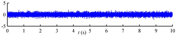
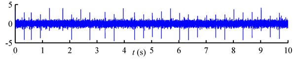
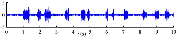
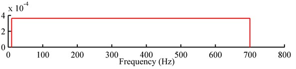
According to Rouillard [4, 19] and Rizzi [12], non-Gaussian random vibrations encountered in engineering practice can be roughly classified into two categories: the “steady” type, in which the high-excursion peaks are distributed uniformly over time, as shown in Fig. 1(b); and the “burst” type, in which the high-excursion peaks emerge in clusters over time, as shown in Fig. 1(c). The non-normality of burst non-Gaussian random vibration is attributed to its nonstationary over short durations. However, from long duration point of view, burst non-Gaussian random loadings are always treated as stationary processes [2]. A comparison of standardized Gaussian, steady non-Gaussian and burst non-Gaussian vibration signals with the identical PSD is shown in Fig. 1.

Fig. 1Three types of random loadings with the identical PSD: a) Gaussian; b) steady non-Gaussian; c) burst non-Gaussian; d) PSD

a)

b)

c)

d)

3. Dynamic stress response analysis

3.1. Modal analysis

The subject of this study is the Euler-Bernoulli beam. The stress response of the beam is directly related to the displacement response. Modal analysis is the basis of displacement response calculation. For the constant-section cantilever beam, the $n$ -th bending mode shape is expressed as follows:

5

W_{n} (x) = s i n β_{n} x - s i n h β_{n} x - α_{n} (c o s β_{n} x - c o s h β_{n} x),

where $x$ denotes the position along the axial direction, as shown in Fig. 2. $β_{n} l = D_{n}$ is a constant for specified $n$ , and $l$ is the length of the beam. $α_{n} = (s i n D_{n} + s i n h D_{n}) / (c o s D_{n} + c o s h D_{n})$ , where ‘ $s i n h$ ’ and ‘ $c o s h$ ’ denote the hyperbolic sine function and hyperbolic cosine function, respectively. The modal frequency corresponding to $W_{n}$ is:

6

ω_{n} = {(β_{n} l)}^{2} \sqrt{\frac{E I}{ρ A l^{4}}},

where $E$ is the elastic modulus, $I$ is the moment of inertia of the cross-section, $ρ$ is the density of the material and $A$ is the cross-sectional area. The $n$ -th mode shape $W_{n} (x)$ satisfies the following equation [20]:

7

E I \frac{d^{4} W_{n} (x)}{d x^{4}} = ω_{n}^{2} ρ A W_{n} (x) .

3.2. Displacement response

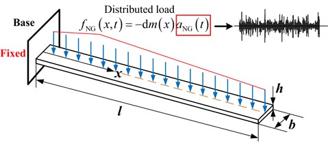
A schematic view of the cantilever beam subjected to non-Gaussian random base excitation $a_{N G} (t)$ , is shown in Fig. 2 where $a_{N G} (t)$ is acceleration signal. For stress response analysis, only the calculation of relative motion is needed. And in this sense, the dynamic system shown in Fig. 2 is equivalent to that show in Fig. 3 in light of the theory of base excitation [20]. The distributed load shown in Fig. 3 is determined by the distributed mass of the beam, $d m (x)$ and the non-Gaussian base excitation $a_{N G} (t)$ . And $d m (x)$ in Fig. 4 is defined as follows:

8

d m (x) = ρ A d x .

Fig. 2Schematic view of cantilever beam subjected to non-Gaussian random base excitation

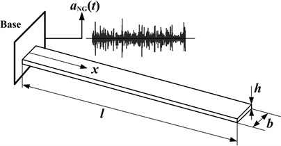
Fig. 3Equivalent dynamic system to that shown in Fig. 2 for stress response analysis

According to Fig. 3 and Eq. (5), the generalized force corresponding to the $n$ -th mode is:

9

Q_{n} (t) = \int_{0}^{l} f_{N G} (x, t) W_{n} (x) d x .

Because the distributed load $f_{N G} (x, t)$ can be recognized to be applied on the central line of constant section beam, as shown in Fig. 3, then the generalized forces corresponding to torsional modes are all equal to zero. Based on the mode superposition method, the transverse displacement at position $x$ is:

10

w (x, t) = \sum_{n = 1}^{\infty} W_{n} (x) q_{n} (t),

where $q_{n} (t)$ is the generalized displacement corresponding to $W_{n} (x)$ . The differential equation of the cantilever beam is:

11

E I \frac{\partial^{4} w (x, t)}{\partial x^{4}} + ρ A \frac{\partial^{2} w (x, t)}{\partial t^{2}} = f_{N G} (x, t) .

Substituting Eq. (10) into Eq. (11), results in:

12

E I \sum_{n = 1}^{\infty} \frac{d^{4} W_{n} (x)}{d x^{4}} q_{n} (t) + ρ A \sum_{n = 1}^{\infty} W_{n} (x) \frac{d^{2} q_{n} (t)}{d t^{2}} = f_{N G} (x, t) .

According to Eq. (7), Eq. (12) can be rewritten as follows:

13

\sum_{n = 1}^{\infty} ω_{n}^{2} W_{n} (x) q_{n} (t) + \sum_{n = 1}^{\infty} W_{n} (x) \frac{d^{2} q_{n} (t)}{d t^{2}} = \frac{f_{N G} (x, t)}{ρ A} .

Based on the orthogonality condition, and multiplying Eq. (13) by $W_{m} (x)$ , $m =$ 1, 2, ..., $\infty$ , and integrating over [0, $l$ ] results in:

14

\frac{d^{2} q_{n} (t)}{d t^{2}} + ω_{n}^{2} q_{n} (t) = \frac{1}{ρ A b_{n}} Q_{n} (t),

where $b_{n} = {‖W_{n} (x)‖}_{2}^{2} = \int_{0}^{l} W_{n}^{2} (x) d x$ is a normalized parameter. Eq. (14) can be treated as the forced vibration differential equation of an undamped SDOF system. $q_{n} (t)$ is obtained by a convolution integral:

15

q_{n} (t) = \frac{1}{ρ A b_{n} ω_{n}} \int_{0}^{t} Q_{n} (τ) s i n (ω_{n} (t - τ)) d τ .

The transient response driven by the initial condition is neglected. Introducing $n$ -th modal damping ratio $ζ_{n}$ into Eq. (15) yields:

16

q_{n} (t) = \frac{1}{ρ A b_{n} ω_{n}^{(d)}} \int_{0}^{t} Q_{n} (τ) e^{- ζ_{n} ω_{n} (t - τ)} s i n ω_{n}^{(d)} (t - τ) d τ,

where $ω_{n}^{(d)} = ω_{n} {(1 - ζ_{n}^{2})}^{1 / 2}$ is the $n$ -th resonant frequency.

By substituting Eq. (16) into Eq. (10), the dynamic displacement response can be expressed as follows:

17

w (x, t) = \sum_{n = 1}^{\infty} [W_{n} (x) \frac{1}{ρ A b_{n} ω_{n}^{(d)}} \int_{0}^{t} Q_{n} (τ) e^{- ζ_{n} ω_{n} (t - τ)} s i n ω_{n}^{(d)} (t - τ) d τ] .

Note that the contribution of the $n$ -th mode to the displacement response decreases with the increase of modal frequency $ω_{n}$ . Normally, accounting for the first three or first four modes can always guarantee accuracy. In this study, the first four modes are taken into consideration. The parameters ${β_{n}}$ in Eq. (5) satisfy [21]:

18

β_{1} l = 1.8751, β_{2} l = 4.6941, β_{3} l = 7.8548, β_{4} l = 10.9955 .

By taking only the first four modes into consideration, Eq. (17) can be rewritten as follows:

19

w (x, t) = \sum_{n = 1}^{4} [W_{n} (x) \frac{1}{ρ A b_{n} ω_{n}^{(d)}} \int_{0}^{t} Q_{n} (τ) e^{- ζ_{n} ω_{n} (t - τ)} s i n ω_{n}^{(d)} (t - τ) d τ] .

3.3. Stress response

The dynamic bending stress at position $x$ is associated with the bend radius. The maximum bending stress occurs at the surface of the beam. For fatigue analysis, the maximum bending normal stress at position $x$ is expressed as follows:

20

σ (x, t) = \frac{E h}{2 υ (x, t)},

where $h$ is the thickness of the beam (as shown in Fig. 2) and $υ (x, t)$ denotes the bend radius of the beam at position $x$ and instant $t$ . The bend radius is defined by the following equation:

21

\frac{1}{υ (x, t)} = \frac{\frac{d^{2} w (x, t)}{d x^{2}}}{{[1 + {(\frac{d w (x, t)}{d x})}^{2}]}^{3 / 2}} .

Substituting Eq. (21) into Eq. (20), the dynamic stress response is expressed as follows:

22

σ (x, t) = \frac{E h \frac{d^{2} w (x, t)}{d x^{2}}}{2 {[1 + {(\frac{d w (x, t)}{d x})}^{2}]}^{3 / 2}} .

Substituting Eq. (19) into Eq. (22) produces:

23

σ (x, t) = \frac{E h \sum_{n = 1}^{4} [\frac{d^{2} W_{n} (x)}{d x^{2}} \frac{1}{ρ A b_{n} ω_{n}^{(d)}} \int_{0}^{t} Q_{n} (τ) e^{- ζ_{n} ω_{n} (t - τ)} s i n ω_{n}^{(d)} (t - τ) d τ]}{2 {[1 + {(\sum_{n = 1}^{4} \frac{d W_{n} (x)}{d x} \frac{1}{ρ A b_{n} ω_{n}^{(d)}} \int_{0}^{t} Q_{n} (τ) e^{- ζ_{n} ω_{n} (t - τ)} s i n ω_{n}^{(d)} (t - τ) d τ)}^{2}]}^{3 / 2}} .

Note that the expression for the stress response (Eq. (23)) is more complex than that for the displacement response (Eq. (19)). Based on Eq. (23), we can analyze the factors influencing the output kurtosis for a given mechanical structure. These factors mainly include the non-Gaussian character (steady or burst), input kurtosis, input bandwidth, modal damping ratio. In this study, attention has been focused on the following three factors: non-Gaussian character, input kurtosis and input bandwidth, as illustrated in the following examples.

4. Numerical examples

A cantilever beam made of aluminium alloy, Al 2024-T3, is selected as the object in the following two numerical examples. The parameters of the material are listed in Table 1. The dimensions are $l =$ 500 mm, $b =$ 20 mm, and $h =$ 2 mm.

Table 1The mechanical properties of Al 2024-T3

Elastic modulus (GPa)	Poisson ratio	Ultimate stress (MPa)	Density (kg/m³)
68	0.33	438	2770

The first four mode shapes can be calculated from Eq. (5). The modal frequencies are derived theoretically (Eq. (6)) and obtained with finite element analysis (FEA) software. The results are listed in Table 2. The differences between the theoretical results and those from FEA software are negligible. The theoretical results are adopted in this study for the completeness of the theoretical analysis, but for complex structures, the FEA software can offer a good substitute.

Table 2The first four mode frequencies of the cantilever beam

Method	Modal frequency (Hz)
Method	First	Second	Third	Fourth
Theoretical	6.41	40.16	112.36	219.69
FEA	6.42	40.25	112.71	220.93

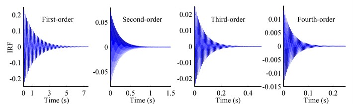
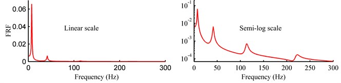
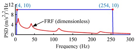
From Eq. (14), the generalized differential equation of the $n$ -th mode can be equivalent to the equation of an SDOF system. The generalized impulse response functions (IRFs) of the first four modes are shown in Fig. 4(a). The frequency response function (FRF) is obtained by summing the IRFs and conducting the Fourier transformation, as shown in Fig. 4(b). The modal damping ratio is assumed to be $ζ_{n} =$ 0.02 based on the properties of Al 2024-T3.

Fig. 4The IRFs and FRF of the cantilever beam: a) IRFs of the first four modes; b) FRF on linear scale and semi-log scale, respectively

a)

b)

4.1. Input base excitations

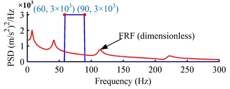
Two numerical examples representing different practical situations are provided. For each example, the input base excitations are Gaussian, steady non-Gaussian and burst non-Gaussian random vibrations with the identical PSD. The input PSDs for the two examples are shown in Fig. 5(a) and Fig. 5(b), respectively. As shown, the input bandwidth in the first example covers the first four modal frequencies, and that in the second example is located between the second and third modal frequencies. These two examples represent two typical situations encountered in engineering practice. In the first example, the RMS value of the three kinds of base excitations is 50 m/s² (5 g). In the second example, the input RMS value is 300 m/s² (30 g). The input kurtosis values are $K_{i n} =$ {4, 6, 8, 10} for the non-Gaussian random excitations in these two examples. Thus, one Gaussian, four steady non-Gaussian and four burst non-Gaussian base excitations will be analyzed in each example. Additionally, if the vibration is in vertical direction, the stress induced by gravity should be taken into consideration. But in this study, we will just focus on the normal situation to study the response behavior of linear structure under non-Gaussian base excitations.

Fig. 5The PSDs of the random base excitations: a) example 1; b) example 2

a)

b)

4.2. Example 1

The PSD of the Gaussian and non-Gaussian random base excitations is shown in Fig. 5(a). The frequency range covers the first four modal frequencies. The stress responses are derived based on Eq. (23). Although, we can calculate the stress response at any location of the beam from Eq. (23), for fatigue analysis, we just need concern the point where the max stress response occurs. It is clear that the max stress point is the fixed end of the cantilever beam. The stress concentration factor at the fixed end of the beam is 1.3694 based on the analysis with FEA software. Then, the response statistics can be estimated from the calculated stress time histories. The output stress RMS and kurtosis at the fixed end to every random excitation are compared in Fig. 6(a) and Fig. 6(b), respectively.

As shown in Fig. 6(a), the output stress RMS values corresponding to Gaussian, steady non-Gaussian and burst non-Gaussian base excitations are approximately consistent disregarding non-normalities of the non-Gaussian inputs. Additionally, the output RMS values hardly change with the increase of the input kurtosis values, $K_{i n}$ for the non-Gaussian loadings. And the small fluctuations of output RMS values along $K_{i n}$ can be attributed to the statistical error from the excitations itself with limited time duration.

As shown in Fig. 6(b), the output stress kurtosis values $K_{o u t}$ corresponding to Gaussian, steady non-Gaussian and burst non-Gaussian base excitations are different. The $K_{o u t}$ value to Gaussian excitation approaches three. However, $K_{o u t}$ values to steady non-Gaussian excitations are somewhat less than three, regardless of the fact that the input kurtosis values, $K_{i n}$ is larger than three. The high-kurtosis diminished from input base excitation to output stress response because the input bandwidth covers the first four peaks of the FRF (Fig. 5(a)), where the first is dominant, and it functions as a filter. After being filtered, the output stress responses tend to sinusoidal curves whose kurtosis is 1.5. For the burst non-Gaussian random base excitations, the output kurtosis $K_{o u t}$ is larger than three but less than the input value $K_{i n}$ . The attenuation of the kurtosis is due to that the linear superposition during the response derivation has smoothed the local non-stationary in the burst non-Gaussian vibrations. However, the kurtosis can transfer to some extent. Phenomenologically, the conclusion is that the non-Gaussian property will attenuate from non-Gaussian (steady and burst) base excitations to stress responses when the input bandwidth covers the modal frequencies.

Fig. 6Output RMS and kurtosis values corresponding to Gaussian, steady non-Gaussian and burst non-Gaussian base excitations with different input kurtosis in example 1: a) RMS; b) kurtosis

Output RMS and kurtosis values corresponding to Gaussian, steady non-Gaussian and burst non-Gaussian base excitations with different input kurtosis in example 1: a) RMS; b) kurtosis

a)

b)

4.3. Example 2

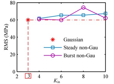
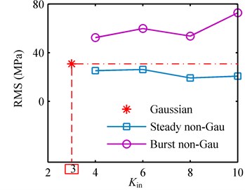
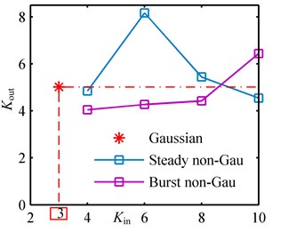
The PSD of the Gaussian and non-Gaussian random base excitations is shown in Fig. 5(b), and the bandwidth is located between the second and third modal frequencies. The stress responses are derived based on Eq. (23). The stress concentration factor at the fixed end of the beam is 1.3694 as mentioned in subsection 4.3. The output stress RMS and kurtosis at the fixed end to every random excitation are compared in Fig. 7(a) and Fig. 7(b), respectively.

As shown in Fig. 7(a), the output stress RMS values corresponding to Gaussian, steady non-Gaussian and burst non-Gaussian base excitations are very different. The variation of output RMS is very different from that in example 1. This is attributed to the change of input bandwidth. The output RMS values corresponding to burst non-Gaussian excitations are much larger than those from Gaussian and steady non-Gaussian cases. The interesting phenomenon is that the output stress RMS values corresponding to steady non-Gaussian excitations are smaller than that from Gaussian case in this example.

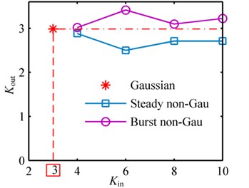
As shown in Fig. 7(b), the output kurtosis values to Gaussian, steady non-Gaussian and burst non-Gaussian base excitations are different. To all the base excitations, the output kurtosis values, $K_{o u t}$ are greater than three. This is different from the usual assumption that Gaussian input results in Gaussian output. The output kurtosis values $K_{o u t}$ to steady non-Gaussian random excitations are smaller than that to Gaussian excitation. However, the output kurtosis values $K_{o u t}$ to the burst non-Gaussian excitations are larger than the Gaussian case. Furthermore, for any kind of non-Gaussian excitation, the output kurtosis values change irregularly along the axis of input kurtosis $K_{i n}$ . Finally for this example, the conclusion is that the stress responses to Gaussian, steady non-Gaussian and burst non-Gaussian random base excitations may be very different in the respect of RMS value and kurtosis value. The burst non-Gaussian base excitations can excite greater stress responses than Gaussian and steady non-Gaussian ones. And it is more destructive. Meanwhile, for steady non-Gaussian based excitations, higher kurtosis does not mean higher output RMS value, higher output kurtosis value and more destructive power.

Fig. 7Output RMS and kurtosis values corresponding to Gaussian, steady non-Gaussian and burst non-Gaussian base excitations with different input kurtosis in example 2: a) RMS; b) kurtosis

a)

b)

4.4. Fatigue life calculation

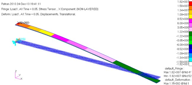
The calculated stress response time histories in example 1 and example 2 are used to calculate the fatigue damage of the cantilever beam under different kinds of base excitations. The toolbox WAFO [22] is used to deal with the time histories. Meanwhile the finite element analysis using MSC.Patran and Nastran is carried out as well for comparison, as shown in Fig. 8. In this study, the rainflow cycle counting method [15] and linear damage accumulation rule [16, 17] are adopted.

Fig. 8The finite element analysis model of the cantilever beam under acceleration base excitation

To predict the fatigue life of the beam, we have estimated the S-N curve of Al 2024-T3 material from constant fatigue test data in three stress levels and it is:

24

N S^{6.34} = 9.4016 \times 10^{19} .

Additionally, according to the research of Benasciutti [1], the rainflow cycles under fatigue limit can still accelerate the fatigue process during random fatigue damage procedure. This assumption is adopted herein. We have calculated the fatigue lives of the cantilever beam according to the stress responses from theoretical calculation and FEA software, respectively.

4.4.1. Fatigue life calculation in example 1

For example 1, the estimated fatigue lives corresponding to different base excitations are tabulated in Table 3. The fatigue life corresponding to Gaussian random base excitation is listed in the last column. The results of steady non-Gaussian random base excitations with different input kurtosis values are listed in the second column and the italicized numbers in parentheses indicate the ratios to Gaussian fatigue life. In the fourth column, the fatigue lives corresponding to burst non-Gaussian base excitations are presented.

Generally, the fatigue life decreases with the increase of the input kurtosis for steady non-Gaussian and burst non-Gaussian cases. When the input kurtosis $K_{i n} =$ 10, the fatigue lives to steady non-Gaussian and burst non-Gaussian random base excitations are approximately 70 % and 60 % that corresponding to the Gaussian loading, respectively. This phenomenon is noteworthy in practice. If non-Gaussianity is neglected, the spectral methods based solely on PSD will overestimate the fatigue life, which is dangerous and fatal in engineering practice. In general, the burst non-Gaussian excitation is more destructive than the steady one based on the data in Table 3.

Meanwhile, the predicted fatigue lives to the entire random base excitations in example 1 based on FEA are tabulated in Table 4. Good agreement is observed between the theoretical results and FEA results.

Table 3Calculated fatigue lives of random base excitations in example 1

$K_{i n}$	Fatigue life (second)
$K_{i n}$	Steady non-Gaussian		Burst non-Gaussian		Gaussian
4	6.2482×10⁵	(0.9493)	5.3937×10⁵	(0.8195)	6.5816×10⁵
6	6.1307×10⁵	(0.9315)	4.1810×10⁵	(0.6352)
8	5.2126×10⁵	(0.7920	1.7071×10⁵	(0.2594)
10	4.4560×10⁵	(0.6770)	3.9007×10⁵	(0.5927)

Table 4Fatigue lives from FEA of random base excitations in example 1

$K_{i n}$	Fatigue life (second)
$K_{i n}$	Steady non-Gaussian		Burst non-Gaussian		Gaussian
4	6.3343×10⁵	(1.0726)	5.3959×10⁵	(0.9137)	5.9056×10⁵
6	5.7993×10⁵	(0.9820)	4.4475×10⁵	(0.7531)
8	4.8379×10⁵	(0.8192)	1.7386×10⁵	(0.2944)
10	4.2951×10⁵	(0.7273)	4.2219×10⁵	(0.7149)

4.4.2. Fatigue life prediction in example 2

For example 2, the estimated fatigue lives corresponding to different base excitations are tabulated in Table 5. The fatigue life corresponding to Gaussian random base excitation is listed in the last column. The results corresponding to steady non-Gaussian random loadings are listed in the second column, and the italicized numbers in parentheses indicate the ratios to Gaussian fatigue life. In the fourth column, the results corresponding to burst non-Gaussian loadings are presented.

Table 5Calculated fatigue lives of random base excitations in example 2

$K_{i n}$	Fatigue life (second)
$K_{i n}$	Steady non-Gaussian		Burst non-Gaussian		Gaussian
4	1.6676×10⁷	(2.3944)	4.1049×10⁵	(0.0589)	6.9645×10⁶
6	6.3439×10⁶	(0.9109)	1.5755×10⁵	(0.0226)
8	6.7284×10⁷	(9.6609)	2.5468×10⁵	(0.0366)
10	5.1902×10⁷	(7.4523)	1.9021×10⁴	(0.0027)

It can be observed that the fatigue lives to the burst non-Gaussian random loadings are much smaller than that to the Gaussian random base excitation. However, for steady non-Gaussian random excitation, the fatigue lives are larger than that of Gaussian case. This can be reflected from the output stress RMS values, as shown in Fig. 7(a). When the input kurtosis $K_{i n} =$ 10, the fatigue life of the burst non-Gaussian excitation is smaller than 4 % that of the Gaussian loading. While for the steady non-Gaussian excitation with $K_{i n} =$ 10, the fatigue life is above 7 times of that to Gaussian case. These results indicate that the higher kurtosis value does not mean higher destructive power. Under the condition described in this example, if non-normalities are ignored, great errors will be introduced both for steady non-Gaussian and burst non-Gaussian cases. In addition, the fatigue lives corresponding to steady non-Gaussian and burst non-Gaussian base excitations are very different. And the burst non-Gaussian base excitation is more destructive than the steady one with identical PSD and kurtosis. This result discloses that the burst non-Gaussian cannot be equated to steady non-Gaussian process during fatigue analysis in practice.

Meanwhile, the predicted fatigue lives corresponding to all the random excitations in example 2 based on FEA are tabulated in Table 6. Good agreement is observed between the theoretical results and FEA results.

Table 6Fatigue lives from FEA of random base excitations in example 2

$K_{i n}$	Fatigue life (second)
$K_{i n}$	Steady non-Gaussian		Burst non-Gaussian		Gaussian
4	1.8824×10⁷	(2.5847)	5.1417×10⁵	(0.0706)	7.2829×10⁶
6	1.3358×10⁷	(1.8342)	5.3893×10⁵	(0.0740)
8	5.5296×10⁷	(7.5926)	2.7020×10⁵	(0.0371)
10	4.0698×10⁷	(5.5881)	1.6532×10⁵	(0.0227)

5. Conclusions

Non-Gaussian random vibrations exist extensively throughout actual environments. These random vibrations can be roughly classified into two categories: steady one and burst one. Non-Gaussian random processes are various, and the spectral method based on PSD cannot obtain reasonable results. Using the cantilever beam as the object, we systematically investigated the stress responses and fatigue lives of a beam under Gaussian and non-Gaussian random base excitations. And comparisons are carried out extensively. Based on the results of this study, the following conclusions can be drawn.

1) The dynamic stress response analysis model for non-Gaussian random base excitations is established. The factors affecting the output kurtosis values are determined as: non-Gaussian characters (steady or burst), input kurtosis values, input bandwidth, and modal damping ratios.

2) When the input PSD covers the modal frequencies, the output stress RMS values corresponding to Gaussian, steady non-Gaussian and burst non-Gaussian random loadings are approximately consistent to one another. And in this condition, the non-Gaussian property will attenuate from non-Gaussian (steady and burst) base excitations to stress responses, especially for steady case. Furthermore, the non-Gaussian (steady and burst) base excitations are more destructive than the Gaussian one with the identical PSD.

3) When the input PSD locates between two adjacent modal frequencies, the output stress RMS values corresponding to Gaussian, steady non-Gaussian and burst non-Gaussian random loadings are very different. The output RMS values to burst non-Gaussian random base excitations are greater than that to Gaussian case with the same PSD. However, for steady non-Gaussian base excitations, the output RMS values are smaller than that to Gaussian case. The output kurtosis values for non-Gaussian (steady and burst) base excitations are irregularly changed with the input kurtosis. Furthermore, in this situation, the burst non-Gaussian base excitations are much more destructive than the Gaussian one. However, the steady non-Gaussian excitations are less destructive than the Gaussian one.

4) Overall, for non-Gaussian base excitations, the steady one is very different from the burst one. Higher input kurtosis does not mean higher output kurtosis and higher destructive power than Gaussian base excitation during non-Gaussian vibration analysis. Generally, the burst non-Gaussian base excitation is more destructive than the steady non-Gaussian and Gaussian cases. But for steady non-Gaussian case, the comparative relationship is uncertainty. This discloses that the burst non-Gaussian vibrations cannot be equated to steady non-Gaussian process, and non-Gaussian vibrations cannot be equated to Gaussian ones during fatigue analysis in engineering practice.

References

Benasciutti D. Fatigue analysis of random loadings. Ph.D. Thesis, University of Ferrara, Italy, 2004.

Search CrossRef
Benasciutti D., Tovo R. Cycle distribution and fatigue damage assessment in broad-band non-Gaussian random processes. Probabilistic Engineering Mechanics, Vol. 20, Issue 2, 2005, p. 115-127.

Search CrossRef
Kihl D. P., Sarkani S., Beach J. E. Stochastic fatigue damage accumulation under broadband loadings. International Journal of Fatigue, Vol. 17, Issue 5, 1995, p. 321-329.

Search CrossRef
Rouillard V. The synthesis of road vehicle vibrations based on the statistical distribution of segment lengths. Proceedings of 5th Australasian Congress on Applied Mechanics, Brisbane, Australia, 2007, p. 1-6.

Search CrossRef
Rychlik I., Gupta S. Rain-flow fatigue damage for transformed Gaussian loads. International Journal of Fatigue, Vol. 29, Issue 4, 2007, p. 406-420.

Search CrossRef
Winterstein S. R. Nonlinear vibration models for extremes and fatigue. Journal of Engineering Mechanics-ASCE, Vol. 144, Issue 10, 1988, p. 1772-1790.

Search CrossRef
Lu Z., Yao H. L. Effects of the dynamic vehicle-road interaction on the pavement vibration due to road traffic. Journal of Vibroengineering, Vol. 15, Issue 3, 2013, p. 1291-1301.

Search CrossRef
Steinwolf A. Numerical and experimental studies of linear systems subjected to non-Gaussian random excitations. Probabilistic Engineering Mechanics, Vol. 14, Issue 4, 1999, p. 289-299.

Search CrossRef
Wang J. Non-Gaussian stochastic dynamic response and fatigue of offshore structures. Ph.D. Thesis, Texas A&M University, U.S., 1992.

Search CrossRef
Wang X., Sun J. Q. Multi-stage regression fatigue analysis of non-Gaussian stress processes. Journal of Sound and Vibration, Vol. 280, Issue 1-2, p. 455-465.

Search CrossRef
Grigoriu M. Linear models for non-Gaussian processes and applications to linear random vibration. Probabilistic Engineering Mechanics, Vol. 26, Issue 3, 2011, p. 461-470.

Search CrossRef
Rizzi S. A., Przekop A., Turner T. On the response of a nonlinear structure to high kurtosis non-Gaussian random loadings. NASA Technical report, 2013,

Search CrossRef
http://ntrs.nasa.gov/archive/nasa/casi.ntrs.nasa.gov.

Search CrossRef
Benasciutti D., Tovo R. Fatigue life assessment in non-Gaussian random loadings. International Journal of Fatigue, Vol. 28, Issue 7, 2006, p. 733-746.

Search CrossRef
Grigoriu M., Kafali C. Response of linear systems to stationary bandlimited non-Gaussian processes. Probabilistic Engineering Mechanics, Vol. 22, Issue 4, p. 353-361.

Search CrossRef
Rychlik I. A new definition of the rainflow cycle counting method. International Journal of Fatigue, Vol. 9, Issue 2, p. 119-121.

Search CrossRef
Miner M. A. Cumulative damage in fatigue. Journal of Applied Mechanics, Vol. 12, Issue 3, 1945, p. 159-164.

Search CrossRef
Park Y., Kang D. H. Fatigue reliability evaluation technique using probabilistic stress-life method for stress range frequency distribution of a steel welding member. Journal of Vibroengineering, Vol. 15, Issue 1, 2013, p. 77-89.

Search CrossRef
Mendel J. M. Tutorial on higher-order statistics (spectra) in signal processing and system theory: theoretical results and some applications. Proceedings of the IEEE, Vol. 79, Issue 3, 1991, p. 278-305.

Search CrossRef
Rouillard V. On the non-Gaussian nature of random vehicle vibrations. Proceedings of the World Congress on Engineering, London, UK, 2007, p. 1219-1224.

Search CrossRef
Rao S. S. Mechanical vibration, 5th edition. Prentice Hall, New Jersey, 2010.

Search CrossRef
Steinberg D. S. Vibration analysis for electronic equipment. John Wiley & Sons Inc, New York, 2000.

Search CrossRef
Brodtkorb P. A., Johannesson P., Lingren G., Rychlik I., Rydén J., Sjö E. WAFO – A Matlab toolbox for analysis of random waves and loads. Proceedings of 10th International of Shore and Polar Engineering Conference, Vol. 3, 2000, p. 343-350.

Search CrossRef

About this article

Received

15 February 2014

Accepted

27 April 2014

Published

15 May 2014

Keywords

non-Gaussian vibration

base excitation

cantilever beam

rainflow cycle

fatigue life

Acknowledgements

The authors gratefully acknowledge the financial support of the National Natural Science Foundation of China (No. 50905181).

This is an open access article distributed under the Creative Commons Attribution License, which permits unrestricted use, distribution, and reproduction in any medium, provided the original work is properly cited.