Restoring dynamic properties of damaged buildings using pole assignment control method

1. Introduction

It is clear that the structures experience some damages during their useful life. Many factors such as corrosion, fatigues, wind forces, earthquakes, impacts can produce different types of structural damages. During the past decades, a great amount of research regarding the damage detection of structures has been conducted [1-4]. In the earthquake resistant design of buildings a structure with less severe damage is often required to be operational [5]. To improve the performance of such an operational building, damage can be mitigated using sensors, actuators and controllers. Mitigating the seismic responses of major structures such as tall buildings and wind sensitive bridges using control methods has been studied comprehensively over the years [6-8]. Vibration control and health monitoring of civil structures subject to earthquakes and strong winds have been hot areas of research in the recent years. Both vibration control and health monitoring systems contain similar hardware devices such as sensors, data acquisition and data transmission devices. The examples of combination of these two areas of research can be found in the work of Viscardi and Lecce [9], Ray and Tian [10].

In this paper, pole assignment control algorithm is used for damage mitigation. Because of natural frequency reduction during damage, the open loop eigenvalues of a damaged structure exhibit insufficient stiffness. So they should be modified through a feedback controller. In terms of pole assignment control algorithm, a controller will modify dynamic properties of structure by moving the eigenvalues of open-loop damaged system to their initial place. Pole assignment algorithm is one of the most suitable control algorithms which have been studied extensively in the general control literature, Sage and White, Brogan and Ogata [11-13]. Applications of this algorithm in structural control can be found for example in the works of Soong, Amini, Meirovitch, Martin and Soong, Utku [14-22]. Ashokkumar and Iyengar [23] presented a new approach for partial eigenvalue assignment [24-26] and its application to structural damage mitigation. In partial eigenvalue assignment, only some unwanted eigenvalues of the open loop system matrix are modified through a multiple input state or output feedback controller. Therefore less changes in gain matrix and less control efforts are required. In this research, partial pole assignment is used for comparing the effect of restoring only some undesired poles instead of all poles.

2. Pole assignment control method

The equation of motion of a controlled structural system with n degrees of freedom subjected to an earthquake excitation $f_e\left(t\right)$ is:

where $M$, $C$, and $K$ are the mass, damping and stiffness matrices of the structure, respectively, of order $n\times n$. $u$ in Eq. (1) is taken as the relative displacement with respect to the ground and mass matrix $M$ is considered diagonal. Displacement vector $q\left(t\right)=n\times 1$ and $q_i$ is displacement of $i$th floor relative to ground ($i=$1, 2,…, $N$):

Control force vector $u\left(t\right)$ is of order $l$×1, $f_e\left(t\right)$ is the external force vector of dimension $r\times 1$, $L$ and $H$ are $n\times l$ and $n\times r$ location matrices, which define locations of the control forces and the external excitations, respectively. A state-space representation of Eq. (1) can be written as:

where, $\left\{x\right\}$ is state vector of dimension 2$n\times 1$ and:

$2n\times 2n$, $2n\times m$, and $2n\times r$ are the system matrix, control location matrix, and external excitation location matrix, respectively. The matrices $0$ and $I$ in Eq. (5)-(7) denote the zero matrix and identity matrix of size $n\times n$, respectively.

Fig. 1Representation of the poles in the complex plane

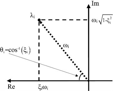
The eigenvalues (poles) of a system represent its dynamic properties. As it is shown in Eq. (8), poles are complex numbers related to the eigenfrequencies and damping ratio. Their graphical representation in complex plane is shown in Fig. 1:

In the state space formulation, these eigenvalues are obtained directly from the eigenvalues of matrix $A$:

The eigenfrequencies $f_i$ and the corresponding damping ratios ${\zeta }_i$ of the uncontrolled system are obtained from the solution of the eigenvalue problem.

It is assumed that control force $u$ is determined by linear state feedback:

where $G$ is $n\times 2n$ gain matrix which is calculated according to the desired eigenvalues (poles) of the controlled system and includes the restoring and damping forces. Replacing the control force $u$ into Eq. (3), the closed loop (controlled) system becomes:

In the above equation system matrix appears as $\left(A-BG\right)$. The new poles of controlled system are defined as eigenvalues of matrix $\left(A-BG\right)$ which are different from eigenvalues of matrix $A$. Such a modification in system matrix by active control causes dynamic properties to be altered.

A control approach chooses gain matrix $G$ in a way that eigenvalues of controlled system have pre-defined values. Such a control method is known as pole assignment control algorithm. A controllable structural system can always be forced to have the desired eigenvalues by choosing an appropriate feedback matrix $G$.

3. Proposed methodology for calculating gain matrix

The pole assignment design consists of selecting the gain matrix $G$ so that the eigenvalues of the controlled system are at the desired locations [13]. In this paper gain matrix is calculated in a way that eigenvalues of undamaged (initial) structure are introduced as desired eigenvalues of the damaged controlled system. Therefore, all eigenvalues of damaged structure will return to their first place in undamaged structure. For this purpose, a simple method to compute gain matrix $G$ is proposed. Deteriorations of stiffness and damping matrix are represented by $\mathrm{\Delta }k$ and $\mathrm{\Delta }c$ respectively. Then the equation of motion of a structural system with n degrees of freedom subjected to an earthquake excitation $f_e\left(t\right)$ in the absence of control force becomes:

Comparing with Eq. (1) which represents the equation of motion of a controlled structural system subjected to an earthquake excitation $f_e\left(t\right)$, the gain matrix $G$ is obtained:

In order to restore all the structural properties, which are lost due to damage, $\mathrm{\Delta }K$ and $\mathrm{\Delta }C$ are considered as:

Indexes 1 and 2 in Eqs. (15) and (16) are related to the undamaged and damaged structure, respectively. Replacing Eqs. (15) and (16) in Eq. (14) the gain matrix is calculated in a way that all poles will return to their first place.

For restoring only some special poles, which have shown less stiffness and damping due to damage, Eqs. (15) and (16) will be changed as:

where $K_3$ and $C_3$ are partial damaged stiffness matrix and partial damping matrix, respectively. They are calculated in a way that only some components of them are supposed to be modified in order to restore some special modal frequencies or damping of the structure. For this purpose two factors of modification are introduced:

In Eqs. (19) and (20), RPMF and IPMF are real part modification factor and imaginary part modification factors, respectively. Index $i$ represents the number of mode and indexes 1 and 2, as mentioned before, are related to the undamaged and damaged structure, respectively. These two factors are used for modifying real and imaginary parts of poles related to $i$th mode and moving them to their first place.

To restore wanted modal damping, the related component of diagonal damping matrix is multiplied by real part modification factor ${\left(RPMF\right)}_i$, since the diagonal components of this matrix (Eq. (22)) are related to modal parameters. Then partial damaged damping matrix is calculated according to Eq. (23):

Similarly, some related components of stiffness matrix are multiplied by imaginary part modification factor ${\left(IPMF\right)}_i$ to restore wanted frequencies. This change is applied through related components of diagonal stiffness matrix. These components are shown as Eq. (25). Then partial stiffness matrix is obtained from Eq. (26):

Following the above procedure and replacing matrix $C_3$ and $K_3$ in Eqs. (17) and (18), gain matrix $G$ can be calculated from Eq. (14).

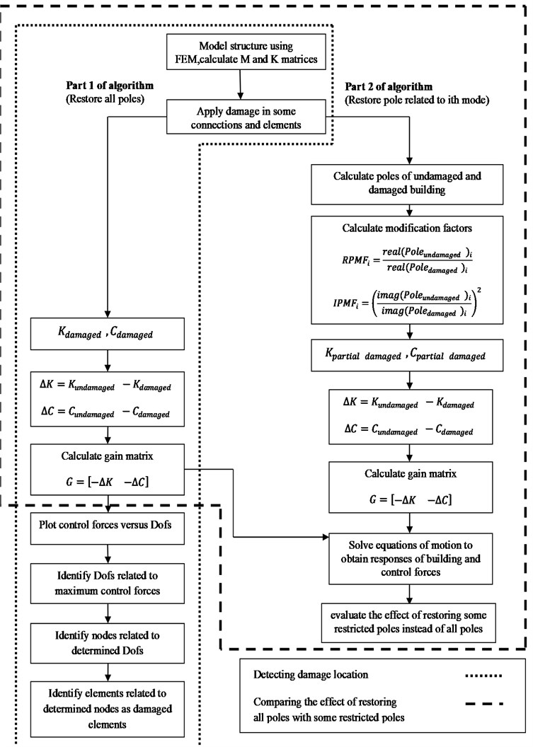
Using the mentioned algorithm and restoring all poles, the location of damaged elements can be verified and restoring only some poles, the effect of each pole is investigated individually. The illustrated investigation steps are shown in Fig. 2.

Fig. 2The steps of investigation for identifying damage location and comparing the effect of restoring some restricted poles instead of all poles using the proposed algorithm

4. Numerical results

In this section, first the proposed algorithm for restoring all poles is applied on a ten-story building with damages in some elements. In this part, verifying damage location is possible considering the location of large control forces. Then the effectiveness of moving undesired poles of damaged building to their first place is investigated. In large structures such as buildings, undesired poles are related to fundamental modes of vibration, since they represent the least stiffness. Three cases of control are applied on the damaged structure. In case 1, all poles are returned to their first place in undamaged building. In case 2, poles related to the first mode and in case 3 poles related to the first and second modes are restored.

For numerical simulation, an example of a 10 story moment-frame building structure is considered. The structure represents a typical concrete moment-frame building which has the masses lumped at each node. The modal damping ratio is uniformly assumed to be 2 % for each mode. Columns have dimensions of 60×60 in the first and second story, 50×50 in the third and fourth story, 40×40 in the fifth and sixth and seventh story, 30×30 in the eighth and ninth and tenth story. All beams have dimensions of 30×30. Damage is applied in some elements by reducing their stiffness. In connections short-length edge elements are defined and their stiffness are reduced to consider damage effect. In this numerical example, the length of edge elements is supposed to be one-tenth of beam or column length. Therefore, the proposed finite element models used for building with damages in connections and elements are different. Fig. 3 shows the proposed finite element models.

Fig. 3Finite element models used for damage in a) elements, b) connections

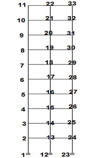
a)

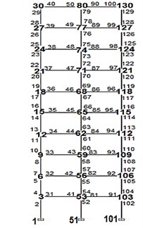
b)

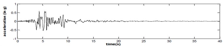
The structure experiences some damages during Newhall earthquake (1971). The ground motion considered is shown in Fig. 4.

Fig. 4Ground acceleration time history for Newhall earthquake (1971)

Three states of damage are defined in the structure. The first state is defined as 30 percent reduction in moment of inertia and 17 percent reduction in area of elements 1 and 21 which are the two edge columns of the first story. The second state of damage is defined as 30, 25, 40, 35 percent reduction in moment of inertia and 17, 14, 23, 20 percent reduction in area of elements 1, 6, 12, 22 respectively. This state of damage is considered to show effectiveness of algorithm in the case of disorganized damage. The third state of damage is related to the damage of connections. This state of damage is defined as 15 % reduction in stiffness of connections, which are related to nodes 3 and 59. The illustrated states of damage are shown in Table 1 and Fig. 5.

Three mentioned cases of control are applied on the three states of damaged structure. The poles of undamaged, damaged and controlled damaged building for each case of control and in each state of damage are shown in Table 2. The bold poles for each case of control are related to restored poles. As it is shown in case 1, 2, 3 all poles, two poles related to first mode and four poles related to first and second mode are moved to their first place in undamaged structure.

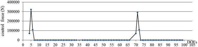
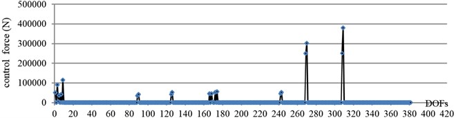
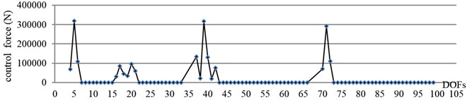
Using the introduced finite element models and applying the mentioned algorithm to restore all poles, the control forces are calculated for three states of damaged structure. The distribution of control forces in the DOFs is shown in Fig. 6. Considering the location of high concentrated control forces, DOFs related to the nodes of damaged elements can be found. For node J, DOF 3J-2, 3J-1 and 3J represent translational and rotational DOFs. Therefore, nodes related to damaged elements can be identified. The elements related to these nodes can be recognized according to Fig. 3. In state 1 of damage large control forces are concentrated in the DOFs related to nodes 2 and 24. The control forces in other degrees of freedom are very low in quantity and can be ignored. As it is shown in Fig. 3, nodes 2 and 24 are the end nodes of elements 1 and 21. So damage location is expected to be in elements 1 and 21. In state 2 of damage, large control forces are concentrated in DOFs related to nodes 2, 6, 7, 13, 14, 24 and 25. These nodes are related to elements 1, 6, 12 and 22. So damage location is expected to be in these elements. In state 3 of damage, large control forces are concentrated in the DOFs related to nodes 2, 3, 4, 31, 43, 58 and 83. So connections related to nodes 3 and 59 are introduced as damaged connections. In this state of damage in Fig. 6, because of more nodes and DOFs in finite element model, the exact number of DOFs related to damaged elements, are not as clear as the two previous states of damage.

Fig. 5Three states of damage which have been considered in the study

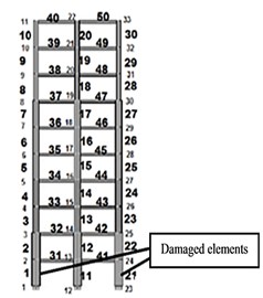
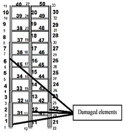
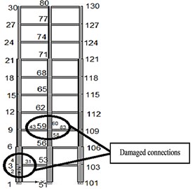
Fig. 6Control forces in each degree of freedom applying: case 1 of control for: a) state1, b) state 2, c) state 3 of damage

a)

b)

c)

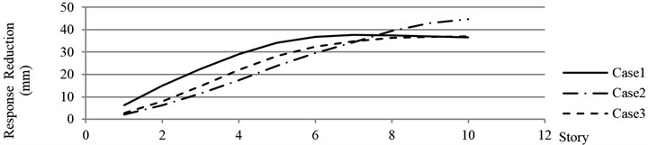
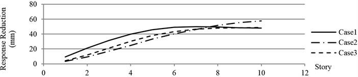
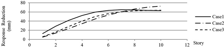
Fig. 7Response Reduction due to three cases of control for: a) state1, b) state 2, c) state 3 of damage

a)

b)

c)

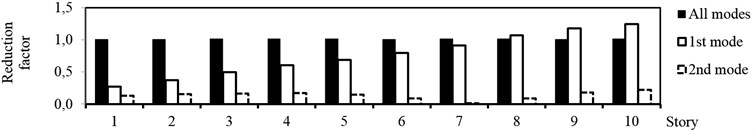
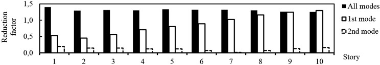
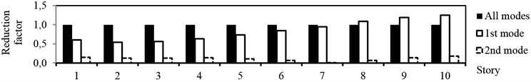
Fig. 8Contribution of all modes, first mode and second mode in total response reduction for: a) state1, b) state 2, c) state 3 of damage

a)

b)

c)

In the next part of this investigation, the effect of restoring only undesired poles instead of all poles is discussed. The relevant controlled results of the damaged system, due to the Newhall earthquake, are compared with the corresponding undamaged and damaged ones in Table 3. Fig. 7 shows response reduction in each case of control for states 1, 2 and 3 of damage. As it is shown in Fig. 7 the changes in response reduction in case 1 of control is more similar to case 3 than case 2. The point is by restoring more poles, the changes in response reductions will be more similar to the case of restoring all poles. The results of response reduction in case 2 of control show that case 2 is more useful case of control for reducing the response of top stories. However, for the lower stories, case 1 and 3 have shown better results for response reductions. So more reduction in responses of top stories can be achieved by restoring only the poles related to the first mode.

For better representation of response reductions due to restoring all poles, poles related to first mode and poles related to second mode, reduction factor is introduced. Reduction factor for each case is defined as the ratio between response reductions of damaged structure due to contribution of poles related to that case of control and total wanted response reductions. Total wanted response reduction in each story is obtained from the difference between damaged and undamaged responses. The reduction factors for the case of restoring all modes, poles related to first mode and poles related to second mode are given in Table 4 and are shown in Fig. 8.

5. Conclusions

In this paper pole assignment control method is applied on a damaged structure. A new control algorithm is proposed for calculating gain matrix in a way that the stiffness/damping characteristics of structure, which have been lost due to damage, can be restored. Using a finite element model and moving all poles of damaged structure to their first place, the location of damage can be verified from the distribution of control forces. A more economical efficient control design can be obtained by restoring some special poles instead of all poles, since fewer changes are applied on the gain matrix and less control effort is required. In the case of restoring all poles, damage location can be verified from the large control forces concentrated to the nodes of damaged elements. In a proper control design, the usage of more control devices with lower capacity is better than fewer control devices with higher capacity. When not all eigenvalues are restored, a more reasonable distribution of control forces can be achievable and more control devices with less capacity are required. So restoring some restricted poles instead of all poles is more useful, especially when some elements have been strongly damaged during an earthquake.

It is important to consider applicability of the proposed technique for a real building. The whole idea of damage mitigation by control method is discussed in this study and a finite element scheme is presented to idealize dynamic behavior of the building. But the authors are studying the applicability of the proposed methodology to a real benchmark model in their next paper.