Stiffness matrix modification with vibration test data by displacement feedback technique

1. Introduction

After spatial discretization by using the finite element method, the equation of motion of a linear elastic time-invariant structure with $n$ degrees of freedom is given by:

In which $M_a\in {\mathbb{R}}^{n\times n}$, analytical mass matrix, is symmetric positive definite and $K_a\in {\mathbb{R}}^{n\times n}$, analytical stiffness matrix, is symmetric positive semidefinite. $\mathbf{q}\left(t\right)\in {\mathbb{R}}^{n\times 1}$ is the displacement vector and $\mathbf{f}\left(t\right)\in {\mathbb{R}}^{n\times 1}$ is the external force vector. Eq. (1) is known as the finite element (FE) analytical model of the structure. Let $\mathbf{q}\left(t\right)=\mathbf{x}{e}^{i\omega t}$ be a soluton of the homogeneous part of Eq. (1), then we can get the following eigenvalue-eigenvector equation:

where ${\lambda }_j={\omega }_j^2$. Let:

where:

Then Eq. (2) can be equivalently written as:

Assume that the modal orthogonality relationship is satisfied:

By substituting Eq. (4) into Eq. (3), we can get another orthogonality relation:

When active control forces are exerted on an undamped vibration system, Eq. (1) now becomes:

where $B\in {\mathbb{R}}^{n\times m}$ is the full column rank control feedback matrix and $\mathbf{u}\left(t\right)\in {\mathbb{R}}^{m\times 1}$ is the control vector. In discussing the feedback control, we assume that the control vector $\mathbf{u}\left(t\right)$ is defined by the control law:

where $F\in {\mathbb{R}}^{m\times n}$ is displacement feedback gain matrix. By substituting Eq. (7) into Eq. (6) yields the following closed-loop system:

Separation of variables by $\mathbf{q}\left(t\right)=\mathbf{y}{e}^{i\omega t},$ which leads to the generalized eigenvalue problems of Eq. (8) as follows:

where ${\sigma }_j={\omega }_j^2$.

In engineering practice, accurate mathematical models are required in order to predict their dynamic characteristics accurately. However, current FE analysis cannot provide sufficiently accurate FE models, which are in good agreement with measured results. A vibration engineer then faces the problem of updating the existing FE model with minimal changes so that the updated FE model can better reflect the measured data from the physical structure being modelled [1]. The updated model may then be considered a better predictions of the responses of the structure, and can be used with greater confidence for damage detection, health monitoring and structural control, and so on.

Model updating techniques are now extensively developed and studied for the structural systems. For undamped systems, to update coefficient matrices using vibration test data by means of direct matrix-updating methods has been considered by Thoren [2], Baruch and Bar-Itzhack [3], Berman and Nagy [4], Wei [5], Modak et al. [6], Yang and Chen [7], Yuan [8], Yuen [9], Yuan and Liu [10], Modak [11] and Sarmadi et al. [12]. For damped structural systems, the theory and methods have been discussed by Friswell et al. [13], Kuo et al. [14], Bai [15], Lancaster [16], Yuan and Dai [17], Yuan and Liu [18] and Mao and Dai [19]. Carvalho et al. [20] presented a numerical method for the stiffness matrix updating problem in an undamped model. by the IMDH (incomplete measured data handling) method, they overcame the difficulty of the incomplete measured data in an algorithmic way without using standard modal expansion or reduction techniques. The method is also capable of preserving the large number of eigendata of the FE model that are not affected by updating. Very more recently, Sehgal and Kumar [21] presented a review of structural dynamic model updating techniques. A number of direct and iterative techniques of model updating along with their applications to real life systems are reviewed and a number of future research directions have been highlighted which can be used for further advancements in the field of model updating.

It is of practical importance for updating an existent model that the newly measured parameters enter the system without altering other unrelated high-order vibration parameters. Such an updating is known as no spill-over. Assume that ${\mathrm{\Lambda }}_1\in {\mathbb{R}}^{p\times p}$, $X_1\in {\mathbb{R}}^{n\times p}$ are known for the first $p$ eigenvalues and associated eigenvectors of the original system. The remaining $n-p$ unknown eigenpairs ${\mathrm{\Lambda }}_2\in {\mathbb{R}}^{(n-p)\times (n-p)}$ and $X_2\in {\mathbb{R}}^{n\times (n-p)}$ remain unchanged. Some explanations for updating with no spill-over being required see the Ref. [32].

The aim of this paper is to modify the stiffness matrix by using the displacement feedback so that the modified second-order system Eq. (8) will contain a number of measured eigenvalues and eigenvectors. Mathematically, the problem of updating stiffness matrix with no spill-over by displacement feedback, therefore, can be stated as follows.

Problem 1. Let $B\in {\mathbb{R}}^{n\times m}$ be a full column rank matrix. Assume that ${\mathrm{\Sigma }}_1=\mathrm{d}\mathrm{i}\mathrm{a}\mathrm{g}\{{\sigma }_1,\cdots ,{\sigma }_p\}\in {\mathbb{R}}^{p\times p}$ and $Y_1=[{\mathbf{y}}_1,\cdots ,{\mathbf{y}}_p]\in {\mathbb{R}}^{n\times p}$ are respectively the measured eigenvalue and eigenvector matrices, where $p\ll n.$ Find displacement feedback gain matrix $F\in {\mathbb{R}}^{m\times n}$ such that:

where $K=K_a+BF$ and $K=K^{{\rm T}}$. Generally, the solution of Problem 1 is not unique. Thus, we need to solve the following least-squares approximation problem.

Problem 2. Find $\widehat{F}\in {\mathbf{S}}_E$ such that:

where ${\mathbf{S}}_E$ is the solution set of Problem 1. Once the solution $\widehat{F}$ of Problem 2 is obtained, the updated stiffness matrix can be expressed as:

Many structural components are generally subjected to dynamic loadings in their working life. Very often these components may have to perform in severe dynamic environment where in the maximum damage results from the resonant vibration [22]. Therefore, in order to avoid the undesired phenomena, one way is to use feedback control so that the unfavorable eigendata are replaced by some suitable ones [23-26]. The idea of using the eigenstructure assignment technique to solve the model updating problem has been considered by [27, 28]. The method can produce an updated FE model on damping and stiffness matrices that matches the measured modal data. More recently, Ouyang and Zhang [29] addressed passive structural modifications of mass-spring systems for partial assignment of natural frequencies, two solution methods were proposed to construct the required mass-normalised stiffness matrix, which satisfies the partial assignment requirement of natural frequencies and maintains the configuration of the original structure after modifications. Sen and Bhattacharya [30] adopted a control theory-based eigenstructure assignment technique to update the FE model of a linear time-invariant system. The proposed method uses state feedback to produce the gain matrix which in turn updates the existing system matrices through simultaneous assignment of eigenvalue and eigenvector pairs in the FE model generated system matrices. Richiedei and Trevisani [31] introduced a novel hybrid method for vibration control in lightly damped systems through the concurrent synthesis of passive structural modifications and active state feedback control gains. The passive modifications alter the set of eigenvectors that can be achieved through state feedback control and gives additional degrees of freedom in the controller synthesis, which overcoming the limitations of eigenstructure assignment through active control used alone.

It should be mentioned that the studies by Zhang et al. [33-35], Chu and Datta [23], Nichols and Kautsky [24], Datta et al. [25] and Lin and Wang [26] lead to a feedback design problem for a second-order control system. That consideration eventually results in either a full or a partial eigenstructure assignment for the eigenvalue problem. Nonetheless, these results cannot meet the basic requirement that the updated matrices should be symmetric. Our main contribution is to provide a new numerical method to solve the FE model updating problem using displacement feedback technique and the updated model has the following properties:

• The measured eigenvalues and eigenvectors will be embedded in the updated model.

• The updated stiffness matrix is also symmetric and positive semidefinite.

• The eigenvalues and eigenvectors corresponding to the unmeasured ones remain unchanged.

• The difference between the updated model and the original model is minimal.

The method directly identifies, without iteration, and works directly on the second-order system model. More importantly, the approach allows the control matrix to be specified beforehand and also leads naturally to a small norm solution of the feedback gain matrices. We believe that the method proposed should give considerable insight into the important model updating problem.

In what follows, in Section 2, by using the QR-decomposition and the singular value decomposition (SVD) of matrices, we provide a necessary and sufficient condition for the set ${\mathbf{S}}_E$ to be nonempty and construct the set ${\mathbf{S}}_E$ explicitly when it’s nonempty. In Section 3, when the set ${\mathbf{S}}_E$ is nonempty, we show that the solution of Problem 2 is unique and present the explicit expression of the unique solution $\widehat{F}$ of this problem. In Section 4, a numerical algorithm is proposed to determine the displacement feedback gain matrix and a numerical example is provided to demonstrate the effectiveness of the proposed method.

As usual, let ${\mathbb{R}}^{m\times n}$ be the set of all $m\times n$ real matrices and $\mathbb{S}{\mathbb{R}}^{n\times n}$ the set of all $n\times n$ symmetric matrices in ${\mathbb{R}}^{n\times n}$. $A^{{\rm T}}\text{,}$$A^{+}$ and $‖A‖$ denote the transpose, the Moore-Penrose generalized inverse and the Frobenius norm of the matrix $A$, respectively. $I_n$ denotes the identity matrix of order $n$.

2. The solution of Problem 1

In order to solve Problem 1, the following two lemmas are needed.

Lemma 1. If $\tilde{Y}\in {\mathbb{R}}^{m\times l}$, $\tilde{Z}\in {\mathbb{R}}^{m\times q}$, then $\tilde{Y}\tilde{N}=\tilde{Z}$ has a solution $\tilde{N}\in {\mathbb{R}}^{l\times q}$ if and only if $\tilde{Y}{\tilde{Y}}^{+}\tilde{Z}=\tilde{Z}.$ In which case, the general solution of $\tilde{Y}\tilde{N}=\tilde{Z}$ can be expressed as $\tilde{N}={\tilde{Y}}^{+}\tilde{Z}+(I_l-{\tilde{Y}}^{+}\tilde{Y})\tilde{L}$, where $\tilde{L}\in {\mathbb{R}}^{l\times q}$ is an arbitrary matrix [36].

Lemma 2. Suppose that $\tilde{A}$, $\tilde{B}\in {\mathbb{R}}^{n\times p}$, then the matrix equation $\tilde{A}\tilde{Y}=\tilde{B}$ has a symmetric solution $\tilde{Y}\in \mathbb{S}{\mathbb{R}}^{p\times p}$ if and only if [37]:

in which case, the general symmetric solution is:

where $\tilde{J}\in \mathbb{S}{\mathbb{R}}^{p\times p}$ is an arbitrary symmetric matrix.

Let:

Assume that the QR-decomposition of $B$ is:

where $Q=[Q_1,Q_2]$ is an $n\times n$ orthogonal matrix ($Q_1\in {\mathbb{R}}^{n\times m}$) and $R$ is an $m\times m$ nonsingular matrix. By Lemma 1 and Eq. (15), Eq. (14) with respect to $F$ is solvable if and only if:

and thus the unique solution can be represented as:

By Lemma 2, Eq. (16) always has a symmetric solution $\mathrm{\Delta }K$ and the general symmetric solution is:

where $S\in \mathbb{S}{\mathbb{R}}^{m\times m}$ is an arbitrary symmetric matrix. Substituting Eq. (18) into Eq. (17), we obtain:

By Eqs. (4) and (5), we get:

Using Eq. (20) and noting that $X_2$ is of full column rank, Eq. (10) is equivalent to:

where $T=M_a^{-1}{K}_a{M}_a^{-1}-X_1{\mathrm{\Lambda }}_1{X}_1^{{\rm T}}$, $P=M_a^{-1}-X_1{X}_1^{{\rm T}}.$ In practice, the matrices $X_2$ and ${\mathrm{\Lambda }}_2$ in Eq. (10) are usually unknown, we notice that the matrices $X_2$ and ${\mathrm{\Lambda }}_2$ don’t appear in Eq. (21) explicitly. It follows from Eq. (21) that:

Observe that:

That is, Eq. (10) is equivalent to:

Substituting Eq. (18) into Eq. (22), we obtain:

which implies that:

Assume that the singular value decomposition (SVD) of $Q_1^{{\rm T}}P$ is:

where $\mathrm{\Theta }=\mathrm{d}\mathrm{i}\mathrm{a}\mathrm{g}\{{\theta }_1,\cdots ,{\theta }_l\}$, ${\theta }_j>0,j=1,\cdots ,l$, $l=\mathrm{r}\mathrm{a}\mathrm{n}\mathrm{k}\left(Q_1^{{\rm T}}P\right).$$U=[U_1,U_2]\in {\mathbb{R}}^{m\times m}$ and $V=[V_1,V_2]\in {\mathbb{R}}^{n\times n}$ are orthogonal matrices, $U_1\in {\mathbb{R}}^{m\times l}$, $V_1\in {\mathbb{R}}^{n\times l}.$

Using Lemma 2 again, the general symmetric solution of Eq. (23) is:

where $H\in \mathbb{S}{\mathbb{R}}^{(m-l)\times (m-l)}$ is an arbitrary symmetric matrix. By substituting Eq. (25) into Eq. (18), we obtain the general symmetric solution of Eqs. (10) and (14) as:

where $H\in \mathbb{S}{\mathbb{R}}^{(m-l)\times (m-l)}$ is an arbitrary symmetric matrix.

Now, to solve Problem 1 is equivalent to finding symmetric matrix $H$ such that:

where $W_1=Q_1{U}_2\text{.}$ Observe that $W_1^{{\rm T}}{W}_1=I_{m-l}\text{,}$ if let $W_2=[Q_1{U}_1,Q_2]\text{,}$ then $W_2^{{\rm T}}{W}_2=I_{n-m+l}$ and $W=[W_1,W_2]\in {\mathbb{R}}^{n\times n}$ be an othogonal matrix. Thus, the equation of Eq. (27) can be equivalently written as:

Let the SVD of $W_1^{{\rm T}}{Y}_1$ be:

where:

are orthogonal matrices, $L_1\in {\mathbb{R}}^{(m-l)\times t}$, $J_1\in {\mathbb{R}}^{p\times t}.$ By Lemma 2, Eq. (29) has a symmetric solution $H$ if and only if:

In which case, the general symmetric solution is:

where $A=M_a{Y}_1{\mathrm{\Sigma }}_1-K_a{Y}_1$ and $G\in \mathbb{S}{\mathbb{R}}^{(m-l-t)\times (m-l-t)}$ is an arbitrary symmetric matrix.

As a summary, we can get the following result.

Theorem 1. Let the QR-decomposition of $B$ be given by Eq. (15) and the SVD of the matrix $Q_1^{{\rm T}}P$ be given by Eq. (24). Assume that $W_1=Q_1{U}_2,W_2=[Q_1{U}_1,Q_2]$ and the SVD of the matrix $W_1^{{\rm T}}{Y}_1$ is given by Eq. (30). If the conditions (28) and (31) hold, then Problem 1 is solvable and the solution set ${\mathbf{S}}_E$ of Problem 1 can be expressed as:

where $P=M_a-X_1{X}_1^{{\rm T}}\text{,}$$A=M_a{Y}_1{\mathrm{\Sigma }}_1-K_a{Y}_1\text{,}$ and $H$ is given by Eq. (32) and $G\in \mathbb{S}{\mathbb{R}}^{(m-l-t)\times (m-l-t)}$ is an arbitrary symmetric matrix.

3. The solution of Problem 2

It has been shown in Section 2 that if the conditions (28) and (31) are satisfied, the solution set ${\mathbf{S}}_E$ is nonempty. Clearly, ${\mathbf{S}}_E$ is a closed convex subset of ${\mathbb{R}}^{m\times n}$. It follows from the best approximation theorem [38] that there exists a unique solution $\widehat{F}$ in ${\mathbf{S}}_E$ such that Eq. (12) holds. Now, we will seek the unique solution $\widehat{F}$ in ${\mathbf{S}}_E$. For $F\in {\mathbf{S}}_E$, we can get:

where $W=[W_1,W_2].$ Thus, by Eq. (32) we can obtain:

where:

Therefore, $‖BF‖=\mathrm{m}\mathrm{i}\mathrm{n}$ if and only if:

By substituting Eq. (34) into Eqs. (19) and (32), we obtain the following result.

Theorem 2. If the conditions (28) and (31) hold, then Problem 2 has a unique solution and it can be described as:

where:

and $H_0$ is given by Eq. (33).

4. A numerical example

Based on Theorems 1 and 2 we can establish an algorithm for solving Problems 1 and 2 as follows.

Algorithm.

1) Input $M_a$, $K_a$, $B$, $X_1$, ${\mathrm{\Lambda }}_1$, ${\mathrm{\Sigma }}_1$, $Y_1.$

2) Compute the QR-decomposition of $B$ by Eq. (15).

3) Compute $P=M_a^{-1}-X_1{X}_1^{{\rm T}}$ and the SVD of the matrix $Q_1^{{\rm T}}P$ by Eq. (24).

4) Compute $W_1=Q_1{U}_2$ and $W_2=[Q_1{U}_1,Q_2],$ and the SVD of the matrix $W_1^{{\rm T}}{Y}_1$ by Eq. (30).

5) Compute $A=M_a{Y}_1{\mathrm{\Sigma }}_1-K_a{Y}_1.$

6) If the conditions (28) and (31) hold, then continue, otherwise, go to 1).

7) Compute $H_0$ and $\widehat{H}$ by Eqs. (33) and (36), respectively.

8) Compute $\widehat{F}$ by Eq. (35).

9) Compute $\widehat{K}$ by Eq. (13).

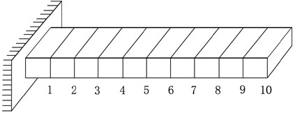
Example. Consider a cantilever beam model (see, Fig. 1). The cross section of the beam is rectangular with length 2 m, width 60 mm and height 3 mm, respectively. The material of the cantilever beam is aluminum alloy with the modulus of elasticity = 71 GPa, Poisson ratio = 0.33 and mass density = 2.714×10^-5 N/mm³$.$ The beam is discretised into 10 elements shown in Fig. 1.

Fig. 1The model of a cantilever beam

The mass matrix of the FE model is diagonal and the stiffness matrix is 3-diagonal, which are given by:

${\mathrm{\Lambda }}_1$ and $X_1$ are given by:

The measured modal data are given by:

Let control feedback matrix $B$ be:

It is easy to check that the conditions (28) and (31) hold:

By the Algorithm, we can obtain the following unique solution of Problem 2:

In which case, the optimal updated stiffness matrix can be figured out.

Fig. 2 indicates the absolute values of the stiffness discrepancy matrix obtained from the proposed model updating method. We define the residual as:

and the numerical results are shown in the Tables 1 and 2.

Fig. 2The absolute values of the stiffness discrepancy matrix (SDM) using the proposed method

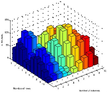
Fig. 3The frequencies of the measured and updated models

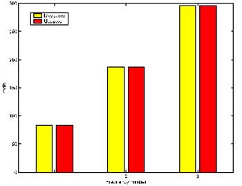
Fig. 4The frequencies of the analytical and updated models

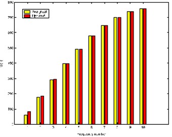
Table 1 shows that the measured modal data are embedded in the new model $M_a{Y}_1{\mathrm{\Sigma }}_1=\widehat{K}{Y}_1$ (Fig. 3 shows the comparison of frequencies of the measured model with the updated model) and Table 2 implies that the model is updated with no spill-over (Fig. 4 shows the comparison of frequencies of the analysis model with the updated model) and the updated stiffness matrix is also symmetric and positive definite.

5. Conclusions

A no spill-over direct updating method for undamped vibration systems with vibration test data using displacement feedback technique has been presented. When the conditions (28) and (31) hold, the required displacement feedback gain matrix can be determined, and the optimal updated stiffness matrix which satisfies the characteristic equation can be achieved. The method is easy to implement, and allows the control matrix to be specified beforehand. Although the proposed method can guarantee that the updated matrix is symmetric and positive semidefinite, it failed to preserve the pattern of the FE stiffness matrix. How to maintain the physical connectivity of the updated matrix is worthy of further study.