Abstract
Vibration signature of flexible structures can be used as a tool to monitor the structural health and predict failure. This work presents a practical low cost technique for predicting vibration signature of a mechanical structure and relates it to its structural health. The technique utilizes a model constructed from Modal frequencies and Eigen vectors obtained via finite element analysis (FEA) of the structure. Linear Quadratic Gaussian (LQG) servo controller of the acceleration output of the model is utilized to minimize error between actual acceleration measurements and its estimates. The LQG controller requires minimal feedback measurements from the physical system and can provide acceleration estimates at any location on the structure. Thus, it is adaptable to structures that are complex and/or have limited accessible measurements points. Anytime during operation, a shift in estimated Modal frequencies of the structure is shown to have a strong relationship with variation in structural parameters, (i.e. structural damage). Therefore, the presented technique is unique for three reasons, (a) it uses estimates, rather than actual measurements to identify structural damage, (b) requires minimal feedback measurements from the structure and (c) uses an effective low-cost reduced order model to achieve (a) and (b). The proposed technique is utilized on a pipeline structure and is evaluated both numerically and experimentally as a proof of concept. Research outcomes are presented and discussed.
1. Introduction
Damage detection in flexible structures using vibration-based methods is the focus of significant research efforts due to its practicality and comprehensiveness. It is elementary that the vibration signature of a structure is tightly related to its material parameters, geometrical dimensions and exogenous forces acting on it. The vibration signature can be thought of as the frequency response of the structure to an exogenous excitation such as impulse forces. Changes in the material, geometrical parameters and excitation, will directly affect its vibration signature [1]. This intimate relation between the structural properties and its vibration signature can be utilized to monitor the structural health and predict any possible failure or damage inflicted on the structure [1-11]. Pipelines are no exception since they usually transport critical fluids that are crucial to everyday living. Some pipelines transport hazardous materials such as oil and natural gas, where failure can have massive implications both environmentally and economically. Therefore, it is critical to maintain the pipeline structure at peak operational readiness. Many nondestructive techniques are available for testing and evaluation of structural health such as eddy current, ultrasound, liquid penetrant, -ray, among others [12-14]. However, those methods are localized methods that are neither globally sensitive to damage nor economically viable as vibration-based methods [15].
In this work, the vibration signature is explored as a viable mean for predicting failure and evaluating the structural health. The relationship between the vibration signature, and material and geometrical properties is exploited to transform health monitoring problem into one that evaluates the natural frequencies and mode shapes of the structure over extended period of time. Therefore, changes in natural frequencies and mode shapes of the structure can be considered as an indication of damage or failure due to changes in material and/or geometrical properties of the structure. However, there are limitations on the ability to obtain an accurate vibration signature either from a model or actual measurements or both. Modeling a structure can be a tedious task especially if the structure is complex, while obtaining useful vibration measurements depends on the ability to retrofit the structure with the needed sensory devices. Examples of such structures are underground pipelines, foundations and subsea infrastructure.
To overcome modeling difficulties associate with complex structures, research work resorts to simplified versions of the structure to generate working models [10, 16-18]. However, this simplication, although works for some applications, it lacks the sensitivity to parameter changes in the structure and might lead to inadequate prediction of the current state of the structure. Other research work depends on models generated from experimental data, such as model identification which is also a viable approach if the experimental data is reliable and it is free of stochastic noise components [1, 2, 4, 19]. Other methods rely on finite element method to generate a working model of the structure which can lead to deficiencies in the model’s ability to predict the behavior of the physical system, especially if the boundary conditions and the element type chosen for the FE model are not properly specified [10, 20, 21].
In this work, problems associated with modeling and sensor placement difficulties are reduced through a series of treatments that yield significant improvement in the ability of the proposed technique to efficiently predict the vibration signature of the structure with good accuracy. Moreover, the accuracy of this proposed technique in predicting the vibration of a structure is extended to achieve improvement of the ability to predict failure from the vibration signature. The proposed technique relies on constructing a preliminary full order model of the structure using Modal frequencies and Eigen functions obtained from FEA. The calculations cost associate with the full order model, which has a relatively large number of degrees-of-freedom, is reduced using Hankel singular value analysis of the modal state energy. Subsequently, a Linear Quadratic Gaussian (LQG) is constructed to improve the model’s performance through feedback of acceleration measurements at some points on the structure. Complexity of pipelines’ structures and their relatively long span could limit the number of sensors that can be placed on it. Therefore, the vibration signature at any location on the pipeline is estimated rather than measured. The latter reduces the need for attaching many sensors to the structure, and allows for estimating the vibration at inaccessible locations, such as underground or subsea sections of the pipeline. The estimates are improved using limited number of measurements as well as the ability of the LQG to generatre optimal estimates of response, with proper tuning. Comparison between the vibration signatures of the healthy pipeline and that of the pipeline after certain time in service can reveal any structural deterioration or damage. Such deterioration will appear in the form of shift in one or more of the Modal frequencies and/or change in the structural mode shapes. The shift in the Modal frequencies or change in mode shapes is a strong indication of failure or damage inflicted on the pipeline. Quantification of this damage is not presented in this work but a preliminary proof of concept is presented instead. This is so because structural deterioration and/or damage are usually random and requires extensive experimental and statistical analysis to establish a working relationship between shift in the frequencies and the type and location of damage. The latter is left for future research work.
This work is organized as follows; first, the formulation of the preliminary full order model is presented in Section 2. In Section 3, the construction of the LQG with its two parts namely, Linear Quadratic Regulator (LQR) and the Kalman-based Linear Quadratic Estimator (LQE), as well as model reduction is briefly presented. Section 4 presents and discusses the outcome of the numerical and experimental work, and presents the effectiveness of the proposed technique in predicting the vibration signature. Section 5 presents the conclusions drawn from this research effort.
2. Structural model and LQG controller
2.1. State-space representation of the pipe system
Considering the nodal coordinates of the pipe’s structure, its dynamics can be described by the second order matrix differential equations:
where q is the nodal displacements vector, is the external input vector, is the nodal output vector, (mass matrix) is positive definite, (damping matrix) positive semidefinite, (stiffness matrix) positive semidefinite, and are the output displacement and output velocity matrices, respectively.
Eqs. (1) and (2) are dimensional, where is the number of nodes in the finite element model. Knowing that is large for large structures, the numerical burden makes difficult to produce a working state-space model suitable for structural estimation and control applications. Thus, dimensional second-order modal model can be used instead, where [22-24]:
where , is the modal matrix, is the diagonal matrix of Modal frequencies, is the modal damping matrix, is the modal input matrix, is modal displacement matrix, and is modal velocity matrix, where and are the number of inputs and outputs, respectively. Thus, the linear, time-invariant (LTI) modal model takes on the form:
Defining a new state vector , the state-space representation of the structure having point forces as the inputs and point accelerations as the outputs is expressed as:
where: and where is the accelerometer locations matrix. Assuming proportional damping then such that and are as defined above. The model constructed in Eqs. (1-8) is the full order modal model of the structure. This is usually a large model if the structure is large with significant number of modes are required to construct a viable model. Thus, the calculations cost associated with implementing such model for vibration estimation and vibration analysis is still high although it is much smaller than the nodal model of Eqs. (1) and (2). Therefore, model reduction is an option provided that accuracy is maintained while reducing mathematical burden. The time-domain linear time-invariant reduced order state-space model of the structure is expressed as:
where such that .
3. Construction of LQG servo controller
After modeling the plant and obtaining the state space matrices of the model given in Eqs. (1-8) for full order model or Eqs. (9-10) for reduced order, the LQG controller can now be designed. The LQG consists of Linear Quadratic Estimator (LQE) and Linear Quadratic Regulator (LQR), [25]. The LQG is usually implemented on digital hardware; therefore, the following is based on discrete-time state-space model.
3.1. LQG structure and closed loop model
For both full and reduced order continuous-time LTI models given above, assuming a zero-order hold (ZOH) and sampling and command updates at time intervals such that , , where is the time, then the linear discrete-time state-space model of the system is expressed as:
where for the full order system, and while for the reduced order model, and . and , are zero mean uncorrelated Process and measurement noise, respectively.
Following the procedure presented in [26], estimated states using Kalman Filter is generated in two steps namely, predictive and update, such that in the predictive step, and before the output is obtained, (i.e. priori estimate), the state estimates and the associated error covariance are expressed, respectively in the form:
After measurement of the output are obtained, the update equations takes on the form:
The difference in Eqs. (14) is called the innovation and is the observer gain. The error between the true state and the estimated values of the states is denoted as such that the state prediction error covariance is . The gain is determined by proper selection of elements of and such that:
and are symmetric matrices whose values are selected depending on the transient response and measurement qualities [27-30].
Assuming that the structure is time-invariant in the sense that the states converge to zero much faster than the parameters can change, the objective of the LQR is to drive the states to zero in an optimal manner. Moreover, we demand that the error goes to zero for best estimates. Since the LQR requires full state feedback and with the availability of the state estimates from the LQE given in the previous section, the associated Riccati equation solution provides the optimal state feedback gain that minimizes the quadratic cost function:
where is positive semi-definite matrix and is positive definite matrix. The state feedback regulator is of type:
It is clear that the feedback given in Eq. (18) will bring the states of the system given in Eq. (11) to zero in an optimal fashion. Since the states of the system have different non-zero initial states, entries of are chosen such that various states are driven to zero at various speeds. Entries of are determined so as to prevent excessively large control moves. If the proposed controller runs for a sufficiently long time, it will yield a stationary Kalman Filter and Regulator for which the values of LQE and LQR gains can be expressed simply by limiting gain values of and , respectively.
3.2. Closed-loop system eigen values and stability
Combining the LQE and LQR is known as the linear quadratic Gaussian (LQG) controller. Examining the stability of the LQE-LQR system, where the combined error and state estimation unforced dynamics of the closed-loop system are expressed by:
Defining a new matrix such that, where matrix is an upper triangular matrix for which the Eigen Values are:
Notice here that the observer gain can be designed independently from the regulator gain by the separation principle [31-33]. In Eq. (20), is the thEigen Value of the corresponding matrix.
If we refer to the closed-loop model of the system dynamics presented in Eq. (19) as the healthy structure, then the Eigen values and Eigen vectors of represent the predicted or estimated Modal frequencies and mode shapes of the structure. We notice that those frequencies are best estimates of those of the structure. This leads to the next concept in this research which is the prediction of any damage or structural parameter changes that might occur after a certain period of time while the structure is in operation. Keeping the LQG servo control gains the same at all times, any change in the structural parameters will alter the actual values of , , and . In that case, a damaged or altered system will have a state-space model of the form similar to the one in Eq. (11) but will be expressed as:
, , and are the previously defined matrices of the damaged system. Therefore, the Eigen values of the closed-loop model of the damaged systems will be:
Notice that the damage to the structure will appear in the in closed-loop model estimated response as shifts in some or all of its Eigen values. The shift is expressed as:
Non zero values of gives a strong indication that the structure has been altered or damaged.
Defining the unforced dynamics of the full-order closed-loop system (CLFOM) and the reduced-order closed-loop systems as and , respectively, and the stability margin as:
Then the CLROM is stable if which is the case if the model is open-loop stable and the controller is designed such that all ’s are within a unit circle; see page 272 of [23]. The following section shows numerically and experimentally that damage inflicted on the structure can be detected from shifts in the natural frequencies predicted by the response of the closed-loop model.
4. Simulation and experimental results
4.1. Finite element model
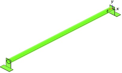
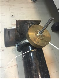
The structure used in this study is an AISI 1020 Low Carbon Steel pipe section shown in Figs. 1 and 2, and has the properties listed in Table 1. The FEA model of the pipe is generated and meshed using ANSYS software package. The latter has 7202 SOLID187, SOLID185 elements and 10966 nodes. Table 2 lists the values of Modal frequencies calculated by ANSYS as-well-as the actual ones obtained from experimental impulse force test of the pipe section. It is clear from Table 2 that FEA Modal frequencies are different from the experimental ones. This is so, for two reasons namely, (a) the FEA model is only a representation of the actual structure and (b) some modes predicted by FEA have negligible contribution to the response in the direction of measurement and/or at the location of sensor placement. Thus, the two aforementioned reasons motivated the use of LQG servo-control and modal reduction to minimize model-plant mismatch.
Table 1Properties of the pipe section
Property | Value | Unit |
Density | 7850 | kg/m3 |
Poisson’s Ratio | 0.29 | – |
Modulus of elasticity | 207 | GPa |
Outer diameter (OD) | 0.10 | m |
Inner diameter (ID) | 0.091 | m |
Thickness () | 0.0055 | m |
Length () | 2.7 | m |
Weight | 27 | kg |
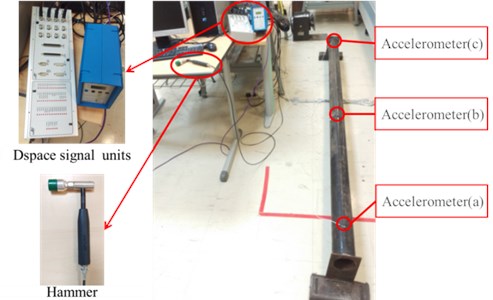
Acceleration measurement is carried out using three PCB uniaxial accelerometers attached to the pipe’s outer surface and have the specs listed in Table 3. All accelerometers measure the acceleration in the -direction which is perpendicular to the ground. Measurement obtained from the Right accelerometer is the only feedback signal to the LQG servo controller. Measurements of Middle and Left accelerometers are only used for evaluating the accuracy of model estimates at the corresponding locations. The targeted outcomes of this work are: 1) Utilize minimal number of physical measurements (Right acceleration) to generate accurate estimates of acceleration at any location on the pipe without the need to place an accelerometer at that location, and 2) Use estimates, instead of actual measurements, to predict variations in structural parameters (i.e. structural failure).
Table 2Numerical and experimental values of the pipe’s Natural frequencies
Mode numbers | Modal frequencies (ANSYS-FEA) | Actual modal frequencies impulse response |
1 | 12 | 12.6 |
2 | 37 | 21.5 |
3 | 71.1 | 73.3 |
4 | 74.8 | 99.7 |
5 | 126 | 111.4 |
6 | 206.1 | 207 |
7 | 334.3 | 209.1 |
8 | 371.54 | 283.1 |
9 | 382.1 | 339.94 |
10 | 432.8 | 413.13 |
Fig. 1Solid model of the pipe section
4.2. Implementation of servo controlled model in -direction
The implementation of the proposed approach is presented in the schematic of the servo controlled closed-loop system shown in Fig. 3. In the following, the input force is applied to the pipe by the instrumented hummer shown in Fig. 2, in the vicinity of the Right accelerometer. Numerical evaluation of the proposed estimation technique is carried out by exciting the structure with multiple hammer hits near the Right accelerometer and collecting the acceleration data at positions a, b and c as indicated in Table 3. A sample input-output data is shown in Fig. 4.
Fig. 2Experimental setup and data acquisition hardware
Data is collected with a dSPACE CP 1104 unit, which also has the closed-loop model built into it. LQR gain vector is determined by proper setting of the elements of for the full-order model and for reduced-order model. The value chosen for since we have one external input to the system. Small value of is chosen to prevent excessive control input to the model. On the other hand, large elements of matrix are designed to bring all the states to the unperturbed state values, faster. Data is collected at a sampling frequency of 10 kHz, which is high compared to the highest considered Eigen frequency of the pipe, but was necessary for the stability of the Matlab Solver handling the numerical calculations. The LQE gain matrix is determined such that the error between estimates and actual is minimized. Entries of are selected to achieve minimal estimation error. Matrix is set to identity since measurement noise is similar for fully functional and identical accelerometers.
Table 3Accelerometer properties and locations relative to the right end of the pipe
Accelerometer designation | Sensitivity (mV/g) | Position label | Distance from right end of pipe |
Right | 99.3 | a | 0.145 m |
Middle | 104.8 | b | 1.121 m |
Left | 101.2 | c | 2.555 m |
Fig. 3Schematic of the servo controlled system used for acceleration estimation
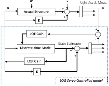
Fig. 4Input-output data from pipe
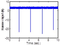
a) Hammer force input
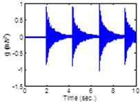
b) Right accel
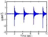
c) Middle accel
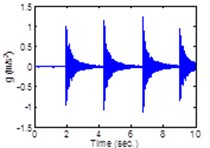
d) Left accel
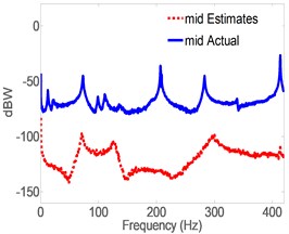
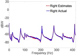
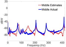
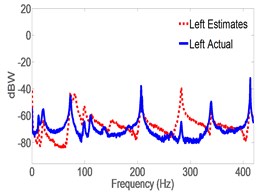
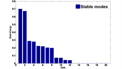
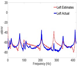
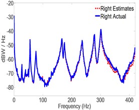
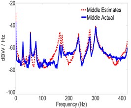
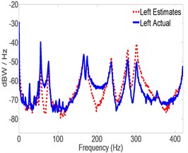
Fig. 5 shows the response spectrum of the open-loop full-order model (OLFOM) to input forces as compared to the actual response of the pipe. It is clear from the Figure, that both Modal frequencies and mode shapes poorly match actual ones. Fig. 6 however, shows that when the LQG servo control is utilized, the closed-loop full-order system (CLFOM) performs better, with clear improvement in estimating modal parameters and mode shapes. Nonetheless, amplitude discrepancies as well as modes that are not in the direction of measurement still appear in the estimates although they might not be detected by actual accelerometer measurement. The tuning values of CLFOM are, , , and , where is the identity matrix. Further improvement to the model is carried out using model reduction based on SVD. To that effect, Hankel Singular Values (HSV) are calculated for the full order model which has a total of 20 states as presented in Fig. 7. The latter shows that only eight states have significant contribution to the response in the direction of measurement, at the three prescribed locations where the output is desired. Therefore, it was found that any state with HSV less than 10 % of the highest value are eliminated without any tangible effect on the accuracy of the model. The closed-loop servo controlled reduced-order model (CLROM) is implemented and the response spectrums at the Right, Middle and Left accelerometer locations are plotted in Fig. 8, this shows that the CLROM outperforms both OLFOM and CLFOM since higher order modes are treated as noise in the CLROM. The values of the estimated Modal frequencies using the CLFOM and CLROM are compared to the actual ones as listed in Table 4, which shows zero estimation error when CLROM is used. The LQG tuning values in this case are, , , and , where is the identity matrix.
Fig. 5Spectrogram of actual vs. estimates of acceleration using full-order model without control
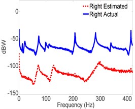
a) Right accel
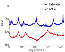
b) Middle accel
c) Left accel
Fig. 6Spectrogram of actual vs. CLFOM acceleration estimates
a) Right accel
b) Middle accel
c) Left accel
Fig. 7Hankel singular values of full-order modal model in y-direction
4.3. Relating changes in structural parameters to modal frequencies shift
The effect of changes in structural parameters on Modal frequencies is examined experimentally based on the two targeted outcomes listed in Section 4.1. All previous simulation results are related to the “healthy” or unaltered pipe. To examine the effect of structural damage on Modal frequencies, a mass block (MB) is retrofitted to the pipe to mimic structural damage such as pipe scale. The pipe retrofitted with the MB is referred to as “damaged” pipe. Further, the effect of damage location relative to sensor location is also tested by varying the MB distance from the feedback sensor along the pipe span. The Right accelerometer measurement is used as the feedback signal to the CLROM and estimates, rather than actual measurement, are used to predict damage. Estimates at the Middle and Left accelerometer locations are generated by the CLROM and frequencies shift in the estimates spectrum, if any, are evaluated, keeping in mind that actual acceleration measurements at the Middle and Left locations are used only to assess the accuracy of CLROM estimates. The MB has a mass of 5.3 kg which is 20 % of the total mass of the pipe. This choice of a relatively high value for the mass block is aimed at eliminating any possibility of experimental error arising from using a smaller mass. To examine the effect of the location of the MB relative to the feedback accelerometer of the Modal frequencies shift, two cases are examined where in Case I the MB is attached at the Left location while in Case II the MB is attached at the middle as shown in Fig. 9. Experiments are carried while using the values of LQG gains for CLROM tuned for the healthy pipe such that Modal frequencies shift predicted by Eq. (23) is examined. The following presents experimental validation of the proposed method.
Table 4Actual modal frequencies of the healthy pipe compared to estimates generated using full-order and reduced-order modal models
Mode Number | Actual (Experimental) (Hz) | Estimated CLFOM (Hz) | Estimated CLROM (Hz) |
1 | 12.69 | 12.3366 | 12.6 |
2 | 21.508 | 21.4851 | 21.5 |
3 | 73.264 | 73.3267 | 73.3 |
4 | 99.6425 | 80.8119 | 99.7 |
5 | 111.3288 | 99.3861 | 111.4 |
6 | 207.0272 | 111.3069 | 207 |
7 | 208.9842 | 149.2871 | 209.1 |
8 | 283.2330 | 206.6733 | 283.1 |
9 | 339.8457 | 208.8911 | 339.94 |
10 | 413 | 282.6337 | 413.13 |
Fig. 8Spectrogram of actual vs. estimates generated by CLROM
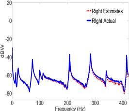
a) Right accel
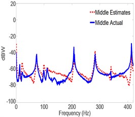
b) Middle accel
c) Left accel
Fig. 9Mass block attached to the pipe
a) MB attached at left “Case 1”end
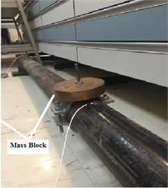
b) MB attached at the middle “Case I1”
4.3.1. Case I: MB attached at the left
In this case, MB was attached to the pipe in the vicinity of the Left accelerometer and acceleration is estimated by CLROM at both left and middle locations. The feedback to the servo controller is the actual acceleration measured by the Right accelerometer. Fig. 10 shows that, estimates of acceleration of the damaged structure have good match to experimental ones and the closed loop system is able to estimate the vibration signature fairly accurately without re-tuning the LQG gains to match the damaged structure. Fig. 11 shows a comparison between estimated acceleration spectrum for both healthy and damaged pipes in which it is clear that shifts are significant in Modal frequencies of Modes 3, 6 and 8, and 9 and 10, as predicted by Eq. (23). Examining the mode shapes of Fig. 11 shows that all the mode shifts are detected in modes that have large displacements in the -direction (i.e. perpendicular to the ground) which is the direction of acceleration measurements. This also validates the effectiveness of the model reduction technique which eliminated all the modes that have minimal contribution to the response in the -direction. Notice that the remaining modes are predominantly in the lateral and horizontal directions, thus sift in their Modal frequencies is minimal in the vertical direction. It should be noticed that in Fig. 11(a), the spectrum is based on actual measurement for both Healthy and damaged because the right accelerometer measurement is available. However, Fig. 11(b) and 11(c) are obtained from estimates only, and thus the shift appearing in Fig. 11(b) and 10(c), are the estimated ones. Table 5 lists the Modal frequencies shift(s) as calculated from the actual Right acceleration measurement’s spectrum in the -direction.
Fig. 10Damaged pipe acceleration estimates vs. actual using CLROM
a) Right end of the pipe
b) Middle of the pipe
c) Left end of pipe
Fig. 11Spectrum of acceleration estimates for healthy and damaged pipes in y-direction. MB at the left location
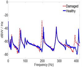
a) Right
b) Middle
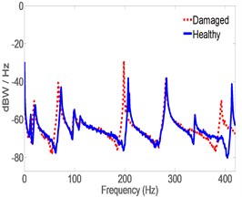
c) Left
Results in Tables 5 and 6 indicate that Modal frequencies found from actual acceleration measurements at the Right are in good agreement with those found from estimates at the Middle and Left. It also shows that the shifts found from estimates are almost identical to those found from actual measurements which is an indication that acceleration estimates are just as reliable as actual ones as per the approach proposed in this work. Fig. 11 and Tables 5 and 6 also indicate that changes in structural parameters can be detected from Modal frequencies estimates using the proposed method. The experiment was replicated three times and the outcome was similar to the results presented, each time. It is worth mentioning that all frequency shifts where towards the left of the graph indicating a drop in the Modal frequencies. This is in-line with expectations since mass was added to the structure. It can also be concluded that a change in stiffness due to cracks or loss of structural continuity would cause a shift in Modal frequencies in the direction of reduced stiffness.
Table 5Modal frequencies shift in the y-direction found from right acceleration spectrum. MB at left
Eigen frequency | (Hz) | (Hz) | ||
Healthy | Damaged | Right Accel. | ×100% | |
12.69 | 11.727 | –0.963 | –7.5 | |
21.508 | 19.532 | –1.976 | –9.186 | |
73.264 | 67.383 | –5.8804 | –8 | |
99.6425 | 98.6712 | –0.9713 | –1 | |
111.3288 | 111.3592 | –0.0304 | 0 | |
207.0272 | 198.2618 | –8.7655 | –4.23 | |
208.9842 | 203.1541 | –5.8301 | –2.7 | |
283.2330 | 282.2200 | –1.0130 | –0.5 | |
339.8457 | 0 | –339.84 | –100 | |
413.0762 | 392.1661 | –20.910 | –5 | |
Table 6Eigen frequency shifts in the y-direction. CLROM estimates at middle and left acceleration spectrums. MB at left
Eigen frequency | (Hz) middle | (Hz) | (Hz) left | (Hz) | ||||
Healthy | Damaged | Middle estimate | ×100 % | Healthy | Damaged | Left estimate | ×100 % | |
12.681 | 11.730 | –0.9517 | –7.505 | 12.6918 | 11.7047 | –0.9871 | –7.784 | |
21.477 | 19.573 | –1.9034 | –8.863 | 21.474 | 19.525 | –1.9488 | –9.074 | |
73.343 | 67.3069 | –6.0366 | –8.231 | 73.317 | 67.352 | –5.9645 | –8.132 | |
99.692 | 98.7137 | –0.9789 | –0.982 | 99.6183 | 98.612 | –1.0061 | –1.009 | |
111.4396 | 111.3580 | –0.0816 | –0.073 | 111.331 | 111.619 | 0.2874 | 0.258 | |
207.1153 | 198.2019 | –8.9134 | –4.304 | 207.0711 | 198.276 | –8.7950 | –4.246 | |
209.025 | 203.1134 | –5.9119 | –2.828 | 209.0186 | 203.176 | –5.8424 | –2.795 | |
283.157 | 282.268 | –0.8889 | –0.314 | 283.1828 | 282.1433 | –1.0395 | –0.367 | |
339.936 | 0 | –339.936 | –100 | 339.939 | 0 | –339.939 | –100 | |
413.1300 | 392.602 | –20.5277 | –4.969 | 413.024 | 392.479 | –20.5445 | –4.973 | |
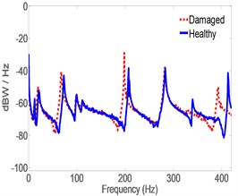
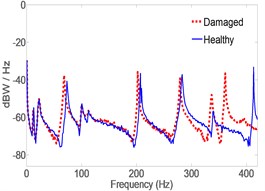
4.3.2. Case II: MB attached at the middle
In this case, MB was attached to the pipe in the vicinity of the Middle accelerometer and estimates where obtained both at the Middle and Left locations using the CLROM while using the Right measurement as the only feedback signal to it. Fig. 12 also shows a clear shift in Modal frequencies due to the MB attachment. However, the nature of the shift and the magnitudes are different from those given in Case I. Tables 7 lists the actual Modal frequencies shift as detected by the Right measurement and its spectrum. Table 8 lists the shift as estimated by the CLROM at the Middle and Left locations. The latter two tables show good agreement between actual and estimated shifts.
4.4. Results analysis
Experimental results have shown that adding MB to the structure has caused modal frequencies shifts in some modes while suppressing other modes. For example Mode 9 in Table 6 and Mode 7 in Table 8 have disappeared when MB was attached to the pipe. This is so because the structural parameters have changed, although the change was a localized one. Modes affected by the addition of MB are those having a mode shape involving bending the - plane such as Modes 3, 6, 7 and 10. Other modes affected are the ones involving rotation about -axis such as mode 8 and 9. It is noticed also that higher order modes are affected more than lower order modes, for example the shift in Mode 10 is –51.67 Hz. The effect of MB on the frequency shift of Mode 10 was half of that when MB was placed at the Left because it was place very close to the modal node.
Fig. 12Spectrum of acceleration estimates for healthy and damaged pipes in y-direction. MB at the middle location
a) Right
b) Middle

c) Left
Table 7Modal frequencies shift in the y-direction found from right acceleration spectrum. MB at middle
Eigen frequency | (Hz) | (Hz) | (healthy) | |
Healthy | Damaged | Right Accel. | ×100 % | |
12.715 | 11.735 | –0.9808 | –7.71 | |
22.4683 | 22.4963 | 0.0280 | 0.12 | |
73.208 | 68.4330 | –4.7753 | –6.52 | |
100.5743 | 99.7478 | –0.8265 | –0.82 | |
112.328 | 111.961 | –0.3673 | –0.32 | |
207.052 | 202.082 | –4.9701 | –2.40 | |
209.08 | 0 | –209.08 | –100 | |
283.186 | 279.232 | –3.9535 | –1.39 | |
339.5704 | 336.53 | –3.040 | –0.89 | |
413.106 | 361.316 | –51.7903 | –12.53 | |
Table 8Eigen frequency shifts in the y-direction. CLROM estimates at middle and left acceleration spectrums. MB at middle
Eigen frequency | (Hz) Middle | (Hz) | (Hz) Left | (Hz) | ||||
Healthy | Damaged | Middle estimate | ×100% | Healthy | Damaged | Left Estimate | ×100% | |
12.6772 | 11.7106 | –0.9666 | –7.62 | 12.7541 | 11.7326 | –1.0215 | –8.01 | |
22.4403 | 22.5047 | –0.0644 | –0.29 | 22.499 | 22.416 | –0.0828 | –0.37 | |
73.2508 | 68.3309 | –4.9199 | –6.72 | 73.2870 | 68.2840 | –5.0030 | –6.83 | |
100.635 | 99.675 | –0.960 | –0.95 | 100.421 | 99.573 | –0.8480 | –0.84 | |
112.314 | 112.11 | –0.200 | –0.18 | 112.293 | 111.869 | –0.4240 | –0.38 | |
207.0092 | 202.2027 | –4.8066 | –2.32 | 207.0043 | 202.183 | –4.8210 | –2.33 | |
208.9692 | 0 | 208.9692 | 100 | 209.0078 | 0 | 209.0078 | 100 | |
283.2269 | 279.354 | –3.8721 | –1.37 | 283.2355 | 279.338 | –3.8967 | –1.38 | |
339.8541 | 336.840 | –3.0133 | –0.89 | 339.8396 | 336.865 | –2.974 | –0.88 | |
413.051 | 361.3789 | –51.6721 | –12.5 | 413.0763 | 361.338 | –51.7378 | –12.5 | |
It is also clear from the Tables 5-8 that the distance between the localized damage and the feedback sensor has affected the spectrum in different ways and thus, in addition to detecting the damage, this method can be used to detect location of the damage relative to the feedback sensor(s), which is important since limited number of sensors are needed for the CLROM. The manner by which the type of damage and its distance from the sensor is determined is not discussed in this research work due to random nature of failure, which will require extensive statistical analysis of the results presented in this work. The distribution of power into frequency components of the signal (Amplitudes) in Fig. 11 and 12 are not discussed in this work but can be utilized as an added indication of the type of damage inflicted on the structure. The reason for not taking the amplitudes into consideration is that the excitation force applied to the structure was applied manually which made it difficult to replicated test conditions. Modal damping is not considered since damping has not been explicitly altered in the experiment. Anti-resonance or zeros of the system has shown shifts as well since the feedback signal location and locations of estimates are at different distances from modal nodes. This work only considered the first ten modes of vibration to construct the state-space model from FEA data. It is well known that the number of modes retained should be determined based on the modal effective mass rather than lower order modes. However, the proposed method can be easily extended to include modes that have a 90 % or more total effective modal mass participation. Therefore, including more modes into the model before reduction will not have any effect on the functionality and the integrity of the proposed method.
5. Conclusions
This work has presented a technique for modeling and estimating the acceleration at any location on a flexible structure using a servo controlled-FEA-based model. The technique also shows that a properly reduced-order model is capable and effective in providing accurate estimates of the vibration signature while reducing numerical cost even in the presence of process and measurement noise. Estimates obtained by the model can be used to predict variation in structural parameters from shift in estimated Modal frequencies. The technique needs minimal actual feedback from the structure and is able to generate accurate estimates, thus reducing the number of physical sensors needed on the structure. A preliminary proof of concept is presented in this work, which shows that shift in modal frequencies can be interpreted as an indication of structural damage. Much work needs to be done in quantifying the relationship between modal parameters’ variations and changes in structural parameters. However, results obtained from this research shows that the proposed method can be further developed to accurately use estimated vibration signature as a viable mean of nondestructive testing and evaluation of structural parameter changes.
References
-
Bao C. X., Hao H., Li Z. X. Integrated ARMA model method for damage detection of subsea pipeline system. Engineering Structures, Vol. 48, 2013, p. 176-192.
-
Bao C. X., Hao H., Li Z. X. Vibration-based structural health monitoring of offshore pipelines: numerical and experimental study. Structural Control and Health Monitoring, Vol. 20, 2013, p. 769-788.
-
Razi P., Taheri F. On the vibration simulation of submerged pipes: structural health monitoring aspects. Journal of Mechanics of Materials and Structures, Vol. 10, 2015, p. 105-122.
-
Shahverdi S., Lotfollahi-Yaghin M. A., Asgarian B. Reduced wavelet component energy-based approach for damage detection of jacket type offshore platform. Smart Structures and Systems, Vol. 11, 2013, p. 589-604.
-
Shi J. X., Natsuki T., Lei X. W., Ni Q. Q. Wave propagation in the filament-wound composite pipes conveying fluid: theoretical analysis for structural health monitoring applications. Composites Science and Technology, Vol. 98, 2014, p. 9-14.
-
Yao Y., Tung S. T. E., Glisic B. Crack detection and characterization techniques – an overview. Structural Control and Health Monitoring, Vol. 21, 2014, p. 1387-1413.
-
Zhou J. H., Sun L., Li H. N. Study on dynamic response measurement of the submarine pipeline by full-term FBG sensors. Scientific World Journal, 2014.
-
Li S. Y., Wen Y. M., Li P., Yang J., Dong X. X., Mu Y. H. Leak location in gas pipelines using cross-time-frequency spectrum of leakage-induced acoustic vibrations. Journal of Sound and Vibration, Vol. 333, 2014, p. 3889-3903.
-
Mostafapour A., Davoudi S. Analysis of leakage in high pressure pipe using acoustic emission method. Applied Acoustics, Vol. 74, 2013, p. 335-342.
-
Schrotter M., Trebuna F., Hagara M., Kalina M. Methodology for experimental analysis of pipeline system vibration. Modelling of Mechanical and Mechatronics Systems, Vol. 48, 2012, p. 613-620.
-
Qarib H., Adeli H. A comparative study of signal processing methods for structural health monitoring. Journal of Vibroengineering, Vol. 18, 2016, p. 2186-2204.
-
Rizzo P., Gulizzi V., Milazzo A. An integrated SHM system based on electromechanical impedance and guided ultrasonic waves. Structural Health Monitoring 2015: System Reliability for Verification and Implementation, Vols. 1-2, 2015, p. 715-722.
-
Rifai D., Abdalla A. N., Ali K., Razali R. Giant magnetoresistance sensors: a review on structures and non-destructive eddy current testing applications. Sensors, Vol. 16, 2016, https://doi.org/10.3390/s16030298.
-
Zhang D. J., Yu Y. T., Lai C., Tian G. Y. Thickness measurement of multi-layer conductive coatings using multifrequency eddy current techniques. Nondestructive Testing and Evaluation, Vol. 31, 2016, p. 191-208.
-
Yan Y. J., Cheng L., Wu Z. Y., Yam L. H. Development in vibration-based structural damage detection technique. Mechanical Systems and Signal Processing, Vol. 21, 2007, p. 2198-2211.
-
Karaiskos G., Papanicolaou P., Zacharopoulos D. Experimental investigation of jet pulse control on flexible vibrating structures. Mechanical Systems and Signal Processing, Vol. 76, Issue 77, 2016, p. 1-14.
-
Martone A., Antonucci V., Zarrelli M., Giordano M. A simplified approach to model damping behaviour of interleaved carbon fibre laminates. Composites Part B-Engineering, Vol. 97, 2016, p. 103-110.
-
Nembhard A. D., Sinha J. K. Comparison of experimental observations in rotating machines with simple mathematical simulations. Measurement, Vol. 89, 2016, p. 120-136.
-
Negash M., Tufa L. D., Ramasamy M. Performance prediction of a reservoir under gas injection using Box-Jenkins model. International Journal of Oil Gas and Coal Technology, Vol. 12, 2016, p. 285-301.
-
Ma B., Shuai J., Liu D. X., Xu K. Assessment on failure pressure of high strength pipeline with corrosion defects. Engineering Failure Analysis, Vol. 32, 2013, p. 209-219.
-
Zhang Z. Strain modal analysis and fatigue residual life prediction of vibrating screen beam. Journal of Measurements in Engineering, Vol. 4, 2016, p. 217-223.
-
El-Sinawi A. H. Vibration attenuation of a flexible beam mounted on a rotating compliant hub. Journal of Systems and Control Engineering, Vol. 218, 2004, p. 121-135.
-
Gawronski W. K. Advanced Structural Dynamics and Active Control of Structures. Mechanical Engineering Series, Vol. 397, 2004.
-
Abushanab W. S. Inexpensive pipelines health evaluation techniques based on resonance determination, numerical simulation and experimental testing. Engineering, Vol. 5, 2013, p. 337-343.
-
Tsai J. S. H., Wu C. Y., Lee C. H., Guo S. M., Su T. J. A new optimal linear quadratic observer-based tracker under input constraint for the unknown system with a direct feed-through term. Optimal Control Applications and Methods, Vol. 37, 2016, p. 34-71.
-
Panigrahi R., Subudhi B., Panda P. C. A robust LQG servo control strategy of shunt-active power filter for power quality enhancement. IEEE Transactions on Power Electronics, Vol. 31, 2016, p. 2860-2869.
-
Ljung L. System Identification Toolbox for Use with MATLAB. 2007.
-
Fassois S. Identification, Model Based Methods. Academic Press, Vol. 10, 2001, p. 673-686.
-
Ljung L. System Identification Toolbox: User’s Guide. Matlab Simulink, 1995.
-
Lewis F. L., Vrabie D. L., Syrmos V. L. Optimal Control of Discrete‐Time Systems. Optimal Control, Third Edition, 1986, p. 19-109.
-
Das S., Halder K. Missile attitude control via a hybrid LQG-LTR-LQI control scheme with optimum weight selection. 1st International Conference on Automation, Control, Energy and Systems, 2014, p. 115-120.
-
Montazeri A., Poshtan J., Choobdar A. Performance and robust stability trade-off in minimax LQG control of vibrations in flexible structures. Engineering Structures, Vol. 31, 2009, p. 2407-2413.
-
Hsiao F. H., Xu S. D., Wu S. L., Lee G. C. LQG optimal control of discrete stochastic systems under parametric and noise uncertainties. Journal of the Franklin Institute-Engineering and Applied Mathematics, Vol. 343, 2006, p. 279-294.
About this article

Authors acknowledge the support of the Petroleum Institute and ADNOC.
