Numerical and experimental verification of finite element mesh convergence under explosion loading

Wang, Iau-Teh

Journal of Vibroengineering

Browse Journal

Submit article

Published: 30 June 2014

Check for updates

Numerical and experimental verification of finite element mesh convergence under explosion loading

Iau-Teh Wang¹

¹Department of Civil Engineering, R.O.C. Military Academy, Kaohsiung, Taiwan, R.O.C.

Cite the article Download PDF

Downloads 1766

Abstract

Explosions inflict severe damage to building structures and threaten national security as well as social stability; their scope of impact and damage level is subject to the energy contained in the shock waves. Explosion testing is limited by the test site and amount of explosive used; a large scale explosion test is not viable. Therefore, numeric analysis is adopted as the preferred research method instead of an actual field test. The application of finite element analysis requires consideration of the complexity of an analysis model and the mesh density. An explosive load violent enough to cause distortion to mesh cannot reveal the actual mechanical behavior and will compromise the convergence and accuracy of the results. The purpose of this study is to analyze the optimal mesh density of the finite elements under an explosive load, in order to explore the element mesh convergence and to compare the results with the experimental. The results of this study can reasonably simulate an explosion effect, achieve the convergence as indicated by calculation results, and provide a foundation upon which future dynamic mechanic studies may establish numerical models. To enhance the calculation accuracy, this study adopts a fluid dynamic analysis program, LS-DYNA, finite element analysis software, to conduct Fluid-Solid Interaction (FSI). A TNT free-field explosion simulation is analyzed for mesh density convergence under an explosive load. The analysis results reveal a pattern where the shock wave diminishes as it moves further away from the explosion point. The results may serve as reference for studies involving the numeric analysis of explosions.

1. Introduction

An explosion is a process in which large amounts of physical or chemical energy are rapidly released, that is, a phenomenon of energy rapidly releasing due to large amounts of energy in a limited volume over an extremely short period of time. The pressure created by an explosion involves a rapid increase in atmosphere; a dynamic pressure, similar to wind pressure, is formed behind the explosion pressure. When explosion pressure reaches a surface, reflective waves form. During this process, part of the energy is delivered to the ground, causing a ground shockwave. When the wave comes into contact with other objects during the delivery process, it produces vibration pressure called an explosion effect. When an object is subject to an explosion effect, tremendous stress waves form from within, compromising the stability of the internal material [1].

Prior to the national security planning and engineering design of demolition, the damage inflicted by an explosion must be carefully evaluated. Explosions constitute a highly nonlinear issue with very complicated mechanical behavior, making it difficult for precise analysis. In most cases, the analysis is conducted by cross-verifying the data and results of numerical simulation analyses acquired from experiments. Explosion testing requires colossal budgets with limited test sites and is inherently dangerous, which means that relevant on-site tests are limited. To avoid possible danger, computer-aided engineering analysis is used so that explosion experiments can be replaced by numerical simulations. However, the reliability of numerical simulation analysis relies on the precision of a model and is subject to the mesh module.

A shock wave is formed in the air during an explosion. Near the blast center, an air shock wave has high speed and strength. These are key parameters in determining the effect of destruction caused by an explosion [2, 3]. Explosion analysis includes experimental analysis and numerical simulation analysis. Acquisition of data from the blast experiments is hard to acquire because a blast experiment is denied to most research institutes due to high budgets, safety concerns and material restrictions. Therefore, most researches concerning blast analysis adopt numerical simulation and compare their results with military blast standards. Bergeron et al. [4] and Wang [5] conducted a series of experiments to analyze the force of land mines against vehicles by detonating 100 g of C-4. Ma et al. [6] simulate a detonation wave transferred underground and studied the impact that spectrum characteristics of a detonation wave bring to a building structure. Crandle [7] studied the delivery rhythm of seismic waves created by a demolition blast, factors affecting vibration strength and the damage inflicted by a demolition blast. Kivity et al. [8] used 3D software to simulate a small scale ammunition depot explosion experiment. The results showed that, free-field blast pressure extreme is about 1/3 that of a surface blast. Also, when simulation data were compared with experimental results, the blast pressure extreme showed a 15 % relative error. Other researchers also found that the predicted values of blast pressure near the blast center had higher errors, and that the relative errors away from the blast center are smaller [9-11].

The finite element method (FEM) is a numerical method widely adopted in various fields of research. Geotechnical engineering often needs to deal with complex geometry, variances in material properties, and nonlinear behavior of materials [12, 13]. FEM is a combination of multiple numerical methods; it reasonably combines the abovementioned features and provides analysis results with comprehensive information about the displacement field and stress field as reference for an engineering design. The FEM divides deformable into a mesh according to their unlimited degree of freedom, thus simplifying them into a limited degree of freedom to enable the research to generate the desired results. The finer the mesh and the larger the number of the element, the higher the accuracy of the analysis will be. However, numerical errors may accumulate. The larger the number of mesh cells, the longer the time required for hardware computation and the more the computation resource is consumed. To concurrently satisfy both accuracy and efficiency of the simulation results, an analysis on the mesh convergence of the finite elements model is needed. Gebbeken and Ruppert [14] in 1999 built an embedded-mesh model. The fluid mesh and the solid mesh were built independently. The fluid mesh adopts a shared common mode, and the solid mesh adopts a contact mode. The coupling of fluid and solid is established by mesh overlapping. They suggest that the solid mesh density should be at least double that of the fluid mesh. Other studies [15-17] have been conducted on the integration of FEM with a deterministic model for explosion analysis. However, the element mesh convergence of potential instability caused by explosions due to layout designation was no in-depth taken into account in these researches.

The dynamic mechanical behavior of explosions mainly concerns about the analysis of the chronicle reaction of a dynamic load, in which on-loading time is short and vibration frequency is high. This is a topic for the dynamic analysis of the instantaneous dynamic. In addition, material, geometry and status are all highly nonlinear [18, 19]. To address the issues concerning the subject of this study, a numerical analysis tool must have the following criteria: (1) possess a characteristic time of loading and response within a millisecond; (2) be adequate for material nonlinearity, geometric nonlinearity and status nonlinearity; (3) allow the simulation of high nonlinear dynamic analysis; (4) be able to handle the issues of material requirements and interface between soft and hard material and (5) be capable of analyzing a great shift or great deformation of material being subject to stress. In consideration of the characteristics and requirement of the nature of the research subject and according to software function analysis and comparison, LS-DYNA, a dynamic mechanics analysis software, best suits the simulation of violent impact and effects from explosion for this study, in terms of its theory, material model, function, status formula and damage standard. It has the advantage of handling nonlinearity and great deformation behavior in a 3-dimensional space structure; this makes it ideal for solving nonlinear topics like high speed impact and explosion. This study uses explosion testing experiment data to cross verify with numerical analysis, and establishes a reasonable mesh density model as the foundation for numerical analysis of the damage and impact resulting from an explosion.

2. Research methods

The primary research method used in this study is cross verification between the experimental and numerical analysis results. Experimental data is compared with numerical simulations; the experimental data is used as reference to verify the numerical simulation reliability. Analysis of finite element mesh convergence under an explosive load is conducted to provide reference for establishing an explosion data analysis model.

2.1. Numerical analysis method

This study mainly applies the basic concept of the FEM to analyze mesh convergence of the dynamic behavior of an explosion. The FEM of LS-DYNA is used in numerical analysis because it simultaneously offers explicit and inexplicit solutions and is based on the coupling of fluid and solid numerical model developed by Lagrangian and Eulerian (Arbitrary Lagrangian-Eulerian, ALE). The fluid dynamic program is based on continuum mechanics theory; it may be used to fully describe the dynamic gaseous behavior of explosions and analyze fluid-solid interactions, including dynamic topics like geometric nonlinearity, material nonlinearity and contact linearity.

2.1.1. Arbitrary Lagrangian-Eulerian method

The Lagrangian descriptive method, also known as the material descriptive method, defines finite element mesh on the analysis subject in a material grid. When material moves or deforms, the element node moves along with the particles of the material. In terms of the mesh, the mass of the element remains unchanged, and the node’s position on an object remains stationary. When an object deforms, the node moves in space along with the object, and the element also deforms accordingly. A benefit of the program is that it precisely describes marginal movement caused by shifting and stress developed by the material; it is ideal for analyzing the deformation process of material, tracking times of material particles and describing shifting and deformation with precision. The shortfall is that the program may terminate computation due to numerical error; when extreme deformation develops on a mesh, the changes of shape and element mesh of the analysis subject are exactly the same, and a negative volume develops from great distortion and deformation of the mesh. Therefore, numerical simulation of explosions is not ideal for this descriptive method.

The Eulerian descriptive method, also known as the space descriptive method, is based on a space grid and the analysis materials are mutually independent. When material moves or deforms, only the material particles move within the mesh accordingly to another element. The method is primarily used to handle the problem of a deformation of material. The benefit is that the mesh system remains fixed and does not create problems under distortion and deformation. It allows for control of the fluid flow and gas expansion. The shortfall is that, when passing through a material interface, the physical ratio of the expanding material in proportion to the mesh is difficult to obtain, and the material margin needs a larger space. Therefore, when developing the element mesh scope, all material space must be included.

The Arbitrary Lagrangian-Eulerian descriptive method has the simultaneous benefits of both the Lagrangian descriptive method and the Eulerian descriptive method. This method not only overcomes the problem of computation termination due to difficulty of numerical computation caused by excessive deformation of the mesh element, but also effectively controls and tracks the movement behavior of the structural boundary. When applied to real-time analysis of fluid-solid integration dynamics, the Eulerian descriptive method is used for fluids and the Lagrangian descriptive method is used for solids. The ALE descriptive method first executes one or several Lagrangian mesh computations. The units of the mesh, at this time, deform as the material flows. Then, Eulerian mesh computation is executed; while the object’s boundary conditions remain unchanged after deformation, the mesh is reassigned for internal units, and the unit variances (such as density, energy and stress tensor) within the deformed mesh and node speed are assigned to the newly defined mesh. This method overcomes the shortfalls of the Lagrangian descriptive method and the Eulerian descriptive method, and allows researchers to tackle the issues of great deformation and shifting from collision, explosion and high speed impact [20-22].

2.1.2. Element type and time integration

LS-DYNA offers diversified element types. It takes into account differences among analysis types and computational methods and allows choices of element types. This study chooses the ALE method and combines a 3-dimensional, 8-node solid element for analysis computation. It is a 3-dimensional solid structure model, and the elements are defined in 8 nodes, where each node is given a level-shifting degree of freedom in $X$ -, $Y$ - and $Z$ -directions. The degree of freedom of velocity and acceleration are also given. In all, there are 9 degrees of freedom for each node. When subject to compressive stress or great deformation, the volume cannot be zero. This type of element is applicable in explicit dynamic analysis [23].

Shock analysis is an issue of short-time dynamics. A differential equation is concerned with derivatives of time and space, and must be able to effectively solve time integration. This type of differential equation is further divided into explicit and implicit time integrations. The explicit type uses a solution for a previously known time to find the solution for the next time. In other words, it uses the vector of a known time to express a new vector. On the other hand, an implicit type uses an iterative method to find a solution. Regular differential equations express time integration as follows [24]:

1

\frac{\partial U}{\partial t} = - \frac{\partial F (U)}{\partial x} = G (U),

2

G^{A V G} = \int G (τ) \frac{d τ}{Δ t},

3

G^{A V G} = ε G^{t + Δ t} + (1 - ε) G^{t},

4

U^{t + Δ t} = U^{t} + Δ t [ε G^{t + Δ t} + (1 - ε) G^{t}] .

In Eq. (4), when $ε = 0$ , then $G^{A V G} = G^{t}$ , which means $G^{A V G}$ may be obtained from the value of the previous time. This is an explicit method. On the contrary, when $ε \neq 0$ , then $G^{A V G}$ must be obtained from the values of the previous time and the next time, and the iterative method must be applied. This method is an implicit type.

In an explicit time integration method, a central difference method is better for computation of nonlinear topic. Its benefit is that it is not required to compute the combination matrix and mass matrix of all elements; only the dynamic equation needs to be solved. Its shortcoming is that the accuracy of the diagonal mass matrix is subject to the effectiveness of element discretion. The central difference method, an explicit method in LS-DYNA, is briefly described below [25].The central difference method assumes the relationships among acceleration, velocity and shifting to be:

5

{\ddot{U}}_{t} = (\frac{U_{t + Δ t} - U_{t}}{Δ t} - \frac{U_{t} - U_{t - Δ t}}{Δ t}) = \frac{1}{Δ t^{2}} (U_{t - Δ t} - 2 U_{t} + U_{t + Δ t}),

6

{\dot{U}}_{t} = \frac{1}{2 Δ t} (- U_{t - Δ t} + U_{t + Δ t}) .

The variance between the above two equations is $Δ t^{2}$ . To find the answer for shifting at the time $t + Δ t$ , consider the dynamic equation for time ( $t$ ):

7

M {\ddot{U}}_{t} + K U_{t} = P (t) .

Apply Eqs. (5) and (6) in Eq. (7):

8

\frac{1}{Δ t^{2}} M U_{t + Δ t} = P (t) - (k - \frac{2}{Δ t^{2}} M) U_{t} - \frac{1}{Δ t^{2}} M U_{t - Δ t} .

Eq. (8) reveals that $U_{t + Δ t}$ is apparently derived from the shifting of the previous time; only the balance conditions at time ( $t$ ) need to be taken into consideration. This is the benefit of explicit time integration. Explosion analysis is an issue of short-time dynamics; it requires a time interval that is very small. Explicit time integration is the primary time integration method in LS-DYNA. This method is a conditional, stable computation method. Therefore, this method is better for analyzing explosion phenomenon.

2.1.3. Control of time-step computation

In the explicit time integration method, time ( $Δ t$ ) must be small to prevent excessive error from occurring during computation; this is the conditional stability of explicit time integration. The amount of $Δ t$ of different types of elements requires different computation methods, related to the element’s length and material’s sound speed. Eq. (9) shows the formula for $Δ t$ used for the elements selected in this study. When computing time $T$ , the program automatically divides $T$ into $T / Δ t$ cycles; therefore, the time required for computation in the program depends a great deal on the amount of $Δ t$ . The amount of $Δ t$ depends on the mesh size. The finer the mesh, the longer the computation time required and the higher the precision.

For solid elements:

9

Δ t_{e} = \frac{L_{e}}{{[Q + {(Q^{2} + c^{2})}^{\frac{1}{2}}]}},

10

Q = \{\begin{array}{l} C_{1} c + C_{0} L_{e} |{\dot{ε}}_{k k}| for {\dot{ε}}_{k k} < 0, \\ 0 for {\dot{ε}}_{k k} \geq 0 . \end{array}

The time-step ( $Δ t$ ) in the central difference method must be smaller than the threshold value; if it is larger than the threshold value, the central difference method value becomes unstable. The criteria for a stable $Δ t$ of the 3-dimensional, 8-node solid element in LS-DYNA are described below:

11

L_{e} = \frac{v_{e}}{A_{e m a x}} .

The wave speed of regular elastic material (fixed bulk modulus) is:

12

c = {[\frac{4 G}{3 ρ_{0}} + {(\frac{\partial p}{\partial ρ})}_{s}]}^{\frac{1}{2}} .

For elastic material with a fixed bulk modulus, it is:

13

c = \sqrt{\frac{E (1 - υ)}{(1 + υ) (1 - 2 υ) ρ}},

where $Q$ is function representation of volume viscosity coefficient $C_{0}$ and $C_{1}$ ; $L_{e}$ is feature length; $v_{e}$ : element volume; ${\dot{ε}}_{k k}$ : strain rate tensor; $A_{e m a x}$ : area measurement of the longest side; $c$ : material sound speed; $ρ$ is mass density; $E$ : Young’s modulus; $G$ : shear modulus; $υ$ : Poisson ratio.

As a result, $Δ t$ is determined by the smallest mesh element. The density of the mesh determines computational precision, stability and computation time. For stability, LS-DYNA manual suggests $α \leq 0.9$ ; for explosion phenomenon, $α \leq 0.67$ [25].

2.2. Explosion test

Numerical model establishment, simulation experiment and parameter analysis need test data for analysis. The purpose of explosion testing is to obtain the air pressure data on TNT detonation in a free-field, and to verify the accuracy of the numerical analysis. This study plans a near-ground aerial blast to obtain the pressure’s maximum value and detonation wave depletion features in the free-field for cross-verification between numerical analysis and the standard empirical formula.

The free-field explosion test as planned uses 1.0 lb (453.593 g) of TNT, and a blast pressure meter is placed 200 cm from the detonation. The test site is illustrated in Fig. 1. The apparatus used includes a PCB type 137A23 detonation pressure meter. A signal is produced by piezoelectricity, and the maximum detonation pressure measurable is 6,895 kPa. The data capture system includes an oscilloscope and a channel signal regulator. The signal produced by the detonation pressure meter is sent to the oscilloscope through the channel signal regulator. When the detonation pressure exceeds 5 kPa, a signal is recorded.

Fig. 1Layout of free-field blasting site. Explosion test as planned uses 1.0 (lb) of TNT, blast pressure meter is placed 200 cm from the detonation

Fig. 2Schematic diagram of simplified 1/4 model of free-field blast

3. Design of numerical simulation

The results from numerical simulation are influenced by the mesh density and time-step ( $Δ t$ ). Convergence analysis is required prior to establishing a numerical model, in order to obtain the optimal mesh density and time-step.

3.1. Analysis model

This study adopts a numerical simulation method with consideration of fluid-solid interaction, and uses LS-DYNA as the analysis tool to study TNT detonation in a free-field and analyze finite element mesh convergence under a dynamic load. The Eulerian descriptive method is used for dynamite and air numerical models, and the Lagrangian descriptive method is used for the earth to establish numerical analysis models of fluid-solid interaction, in order to conduct convergence analysis of mesh density and time-step.

The analysis model is established with an 8-node solid element. ALE is adopted for computation and the unit is $c m - g - μ s$ . Fig. 2 show the simplified 1/4 model used in the numerical analysis. The air dimension is 260×260×180 (cm), and the air element is defined as an ideal gaseous state. A reflective boundary is set to ‘none’ to simulate an explosion in an infinite area. The TNT setting is rectangular in shape, 1.0 lb (453.593 g) in weight, with 1.63 g/cm³ in density. The dynamite is set at the center of the model at 115 cm above ground. The detonation point is the center of the dynamite. The measurements of soil are 260×260×20 (cm). With the model’s symmetry, 1/4 of the model is used for analysis.

3.2. Material constitutive law and equation of state

The material constitutive law is expressed with a stress tensor and strain tensor; it describes the constitutive law of material constituted with a material phenomenon. Under a static state, stress and strain descriptions are sufficient to express behavioral patterns of material that has been subjected to force. However, if the material strain is excessive, the application of an Equation of State will be needed.

An equation of state (EOS) primarily describes the relations among pressure, temperature, volume, density and internal energy of the material constitutive law. It can also describe the relationship between changes in pressure, a material’s internal energy and density and volume, after being subject to an explosion or collision. For the state of high velocity, high temperature and high pressure from an explosion, the EOS is needed to describe the material’s behavior, in regard to change in volume, to realistically simulate the material’s dynamic response.

3.2.1. Air material models

Table 1 shows the material parameters of air. This study used the MAT_NULL material model to simulate air, and equations of state EOS_LINEAR_POLYNOMIAL were used to describe the material model as in Eq. (14). The ideal-gas equation can be simplified as Eq. (15) (Set $C_{1} + C_{2} + C_{3} + C_{6} = 0$ , and let $C_{4} = C_{5} = γ - 1$ ) [23]:

14

P = C_{0} + C_{1} + C_{2} μ^{2} + C_{3} μ^{3} + (C_{4} + C_{5} μ + C_{6} μ^{2}) E_{0},

15

P = (γ - 1) ρ / ρ_{0} E_{0},

where $E_{0}$ is the internal energy per initial volume, $μ$ is the coefficient of dynamic viscosity, $C_{1}$ , $C_{2}$ , $C_{3}$ , $C_{4}$ , $C_{5}$ , $C_{6}$ are constants, and $V$ is the relative volume, $γ$ is the ratio of specific heats of air, $ρ_{0}$ is the initial value of air density, and $ρ$ is the current air density.

Table 1Material parameters of the air model

$ρ$ (g/cm³)	$E_{0}$ (J/m³)	$V$ (g/cm³)	$C_{4}$	$C_{5}$
1.29	2.5×10⁵	1.0	0.4	0.4

3.2.2. Explosive material models

Table 2JWL and material parameters for TNT explosive model

$ρ$ (g/cm³)	$v_{D}$ (cm/μsec)	$P_{C J}$ (Mbar)	$A$ (Mbar)	$B$ (Mbar)
1.63	0.693	0.21	3.712	0.03231
$R_{1}$	$R_{2}$	OMEGA ( $ω$ )	$V$	$E_{0}$ (J/m³)
4.15	0.95	0.3	1.0	0.07

The MAT_HIGH_EXPLOSIVE_BURN material model was used to simulate the high explosive model. Eq. (16) is the Jones-Wilkins-Lee (JWL) EOS for high explosives [26]. The relevant parameters are shown in Table 2:

16

P = A (1 - \frac{ω}{R_{1} V}) E_{m}^{- R_{1} V} + B (1 - \frac{ω}{R_{2} V}) E_{m}^{- R_{2} V} + \frac{ω E_{0}}{V},

where $A$ , $B$ , $R_{1}$ , $R_{2}$ , and $ω$ are constants pertaining to the explosive, $V$ is the relative volume, $E_{0}$ is the initial energy per initial volume and $E_{m}$ : material internal energy. Table 2: $ρ$ is the mass density, $v_{D}$ is the detonation velocity, $P_{C J}$ is the Chapman-Jouget pressure.

3.2.3. Soil material models

The soil composition model of this study was proposed by Krieg [27]. Taking isotropic plasticity theory as the starting point, there is compressible plasticity in the material. This model can be used in porous material, such as soil, rock and concrete. Based on the above description, the experimental parameters of [5] were used for analysis, and the relevant parameters are given in Table 3.

In the Table 3: $ρ$ is the mass density, $G$ is the shear modulus, $K_{u}$ is the bulk modulus, $a_{0}$ , $a_{1}$ , $a_{2}$ are yield function constant for plastic yield function below, and $P_{c u t}$ is the pressure cutoff for tensile fracture.

Table 3Material parameters of the soil model

$ρ$ (g/cm³)	$G$ (MPa)	$K_{u}$ (MPa)	$a_{0}$	$a_{1}$	$a_{2}$	$P_{c u t}$ (MPa)
1.8	0.000639	0.3	3.4×10^-13	7.03×10^-7	0.3	–6.9×10^-8

4. Results and discussion

This study combines test results and simulation results to discuss the applicability of an optimal mesh density and time-step.

4.1. Numerical mesh convergence analysis

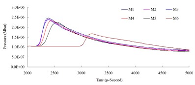
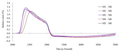
This study used the ALE description method to analyze the coupling effect of fluid and solid. Gebbeken and Ruppert [14] used a modeling method with independent fluid and solid meshes, wherein the fluid mesh used the common point method and the solid mesh used a contact mode; coupling of fluid and solid was established by overlapping the meshes; according to their recommendation, fluid mesh size should be smaller than 1/2 of the size of the solid mesh or, solid mesh density should be at least twice as high as that of the fluid mesh. Therefore, using the TNT edge length as the base for mesh density in the analysis, and because a 1.0 (lb) spherical TNT had the dimensions of 6.56×6.56×9.3 (cm) after being converted into rectangular shape, the dimensions of a simplified 1/4 model would be 3.28×3.28×9.3 (cm). Six simplified 1/4 models of different mesh densities were constructed with mesh edge length equal to 1.0, 0.9, 0.8, 0.7, 0.6 and 0.5 times (represented by M1, M2, M3, M4, M5 and M6) of the TNT edge length; 3D solid 164 solid elements were used to construct a physical model with solid element mesh that’s twice the size of fluid element mesh; the time step scale factor was equal to 0.6. These models were used to conduct mesh density convergence analysis.

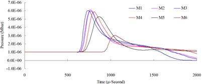
Fig. 3Numerical mesh convergence analysis conducted comparisons of blast pressure at 50 cm from the blast center a) blast pressure duration curve and b) relative error percentages

Numerical mesh convergence analysis conducted comparisons of blast pressure at 50 cm from the blast center a) blast pressure duration curve and b) relative error percentages

a)

b)

The mesh convergence analysis used the numerical model with the highest element mesh density, M6 (element mesh edge length equals to 0.5 times of the TNT edge length), as the base to compare the blast pressures, as well as the relative errors, of numerical models M1-M6 at the same locations. Relative error percentage (%) = (Coarse mesh blast pressure – finer mesh blast pressure) / finer mesh blast pressure × 100 %. Figs. 3-6 show the comparison charts of blast pressure duration curves and blast pressure relative errors at 50, 100, 150 and 200 cm from the blast center.

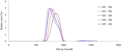
Fig. 4Numerical mesh convergence analysis conducted comparisons of blast pressure at 100 cm from the blast center a) blast pressure duration curve and b) relative error percentages

Numerical mesh convergence analysis conducted comparisons of blast pressure at 100 cm from the blast center a) blast pressure duration curve and b) relative error percentages

a)

b)

Fig. 5Numerical mesh convergence analysis conducted comparisons of blast pressure at 150 cm from the blast center a) blast pressure duration curve and b) relative error percentages

Numerical mesh convergence analysis conducted comparisons of blast pressure at 150 cm from the blast center a) blast pressure duration curve and b) relative error percentages

a)

b)

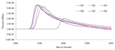
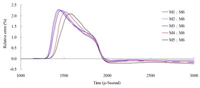
Fig. 6Numerical mesh convergence analysis conducted comparisons of blast pressure at 200 cm from the blast center a) blast pressure duration curve and b) relative error percentages

Numerical mesh convergence analysis conducted comparisons of blast pressure at 200 cm from the blast center a) blast pressure duration curve and b) relative error percentages

a)

b)

The results of the analysis indicated that the blast pressure extremes show a decreasing trend, and that the density of mesh affected the peak values and the decreasing rate. At 50 cm distance from the blast center, only the blast pressure relative error percentage of model M5 fell within a reasonable range; the rest were all greater than 5 %. At 100, 150 and 200 cm from the blast center, the relative error percentages were all smaller than 5 %. This indicated that the numerical model with higher element mesh density has smaller blast pressure relative error than that of lower mesh density. In addition, blast pressures at a close distance to the blast center were greatly affected by mesh density; the results from a low density mesh model were less accurate. The comparison of different mesh dimensions was also conducted to confirm the applicable distance and range of each mesh. According to the analysis result, for the near-field blast effect to be investigated in this research, mesh dimension M6, i.e. mesh edge length equal to 0.5 times of the dynamite’s edge length, was chosen as the base mesh edge length for subsequent blast analysis and time step scale factor analysis.

4.2. Time step convergence analysis

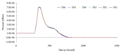
Time step is affected by its scale factor (TSSFAC), as shown in Eq. (17) [28]. A common default scale factor used to calculate time step is 0.9. But, the scale factor should be lowered to 0.67 or less for an explosion or blast numerical analysis to increase the computational stability. Time step scale factor analysis used 6 models with TSSFAC = 0.1, 0.2, 0.3, 0.4, 0.5 and 0.6 (represented by TS1, TS2, TS3, TS4, TS5 and TS6). Blast pressures of each model were compared with that of TS1 to determine a time step scale factor parameter suitable for this study:

17

Δ t = T S S F A C \cdot (l_{m e s h} / C_{l}),

where TSSFAC: time step scale factor; $l_{m e s h}$ : minimum mesh density; $C_{l}$ : wave length.

According to the result of mesh density convergence analysis, mesh with edge length equal to 0.5 times of the dynamite edge length was chosen as the standard mesh for the time step scale factor analysis. To use the TNT edge length as the base for mesh density in the analysis, a 1.0 (lb) spherical TNT was converted into a rectangular shape with dimensions of 6.56×6.56×9.39 cm); thus, the dimensions of a simplified 1/4 model would be 3.28×3.28×9.3 (cm). Using 0.5 times the dynamite edge length as the base, the size of the fluid mesh would be set at 1.64 cm, and the solid mesh set at 3.28 cm. Octahedral solid elements were used to construct a physical model to conduct the time step scale factor convergence analysis.

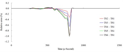
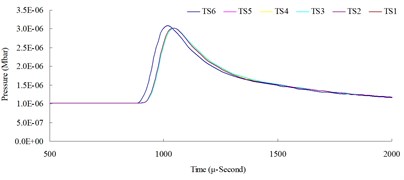
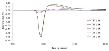
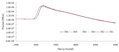
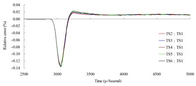
Time step convergence analysis conducted comparisons of blast pressure and relative error to investigate its convergence. Blast pressure of TS1 (TSSFAC = 0.1) was used as the base value to compare the blast pressures of numerical models TS1–TS6 measured at the same distance; also, relative errors were calculated for comparison. Blast pressure relative error percentage (%) = (larger time step scale factor–smaller time step scale factor)/smaller time step scale factor×100 %. Figs. 7-10 show the comparison charts of blast pressure duration curves and blast pressure relative errors at distances of 50, 100, 150 and 200 cm from the blast center, respectively.

Fig. 7Time step convergence analysis conducted comparisons of blast pressure at 50 cm from the blast center a) blast pressure duration curve and b) relative error percentages

Time step convergence analysis conducted comparisons of blast pressure at 50 cm from the blast center a) blast pressure duration curve and b) relative error percentages

a)

b)

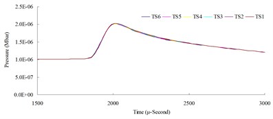
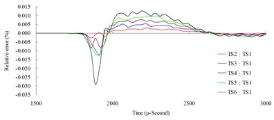
Fig. 8Time step convergence analysis conducted comparisons of blast pressure at 100 cm from the blast center a) blast pressure duration curve and b) relative error percentages

Time step convergence analysis conducted comparisons of blast pressure at 100 cm from the blast center a) blast pressure duration curve and b) relative error percentages

a)

b)

The result of the convergence analysis of time step scale factor (TSSFAC) 0.1–0.6 indicated that scale factor TSSFAC = 0.1 had the longest computation time (11 hrs, 1 min, 27 sec), and TSSFAC = 0.6 had the shortest computation time (1 hr, 58 mins, 18 sec). The relative errors of blast pressures for different time step scale factors, when compared to TSSFAC = 0.1, were all smaller than 1.2 %; the errors fell below 0.1 % as the distance increased. The result of the analysis also showed that the blast pressure duration curves from the scale factor simulation analysis almost overlap each other; no obvious difference was observed.

Fig. 9Time step convergence analysis conducted comparisons of blast pressure at 150 cm from the blast center a) blast pressure duration curve and b) relative error percentages

Time step convergence analysis conducted comparisons of blast pressure at 150 cm from the blast center a) blast pressure duration curve and b) relative error percentages

a)

b)

Fig. 10Time step convergence analysis conducted comparisons of blast pressure at 200 cm from the blast center a) blast pressure duration curve and b) relative error percentages

Time step convergence analysis conducted comparisons of blast pressure at 200 cm from the blast center a) blast pressure duration curve and b) relative error percentages

a)

b)

The above results indicated that time step scale factor had little influence on the blast pressure. Considering the computation time and stability, this study recommends using TSSFAC = 0.3 as the time step scale factor for subsequent research.

4.3. Comparisons numerical analysis with experimental results

According to the results obtained from the study of mesh density and time-step factors, it is confirmed that the element mesh is 0.5 times the side length of the dynamite, and the time-step factor is 0.3. A numerical model for TNT detonation in a free-field is simulated to acquire the explosion history curve. The analysis results are then compared with the experimental results to verify the convergence of the numerical model.

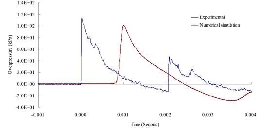
Fig. 11 illustrates the relationship between the blast pressure duration curves from the numerical analysis and experimental result at a measuring point 200 cm from the blast center. The figure reveals that the distribution of the numerical model’s explosion pressure shares the same pattern as that of experimental result. The simulation’s peak blast pressure value of 100.82 kPa had a relative error of – 11.57 % when compared to the experiment’s peak blast pressure value of 114.01 kPa. Relative error percentage (%) = (Blast pressure of numerical analysis – blast pressure of experiment) / Blast pressure of experiment × 100 %. Results from the numerical analysis were consistent with related literature and validated the accuracy [8], as well as the applicability, of the analysis and physical models in this study.

Despite the fact that the numeric results and empirical formulas are not precisely identical and that, due to explosion complexity, the parameters of material and equations of state obtained and summarized from the test are not entirely consistent, the results from the simulation basically conform to objective facts. Therefore, it is confirmed that when an element mesh density is 0.5 times that of the side length of the dynamite and the time-step factor is set at TSSFAC = 0.3, an optimal analysis is allowed for numerical simulation of a free-field TNT explosion.

Fig. 11Blast overpressure duration curves by 1.0 (lb) TNT of experiment and simulation at 200 cm from the blast center

5. Conclusions

When using the FEM for simulation computation, the precision level of the mesh density influences the results of a later study. This study establishes a numerical model of free-field explosions for simulation analysis based on an on-site explosion test. It confirms fluid and solid interaction in explosions and conducts a convergence analysis of mesh density and time-step control criteria. By comparing analysis results and experimental Results, the convergence of the numerical model is verified. The analysis results reveal that analyzing explosion phenomenon using the fluid-solid interaction method enables the study of explosion pressure wave dissemination with better accuracy.

Mesh density convergence analysis indicated that numerical models with higher element mesh density had smaller blast pressure relative errors than the ones with lower mesh density; close-range blast pressures were affected significantly by the mesh density, such that lower density mesh at close range could produce less accurate results. According to the results of the analysis and considering near-field blast effect, element mesh edge length equal to 0.5 times of the dynamite edge length was the better mesh density for the analysis. Time step scale factor convergence analysis produced relative errors smaller than 1.2 %, and the blast pressure distribution curves with various scale factors in the blast pressure distribution chart almost overlapped with each other and showed no obvious difference. Considering the computation time and stability, TSSFAC = 0.3 is recommended as the scale factor for subsequent research. They allow a convergent and stable numerical model and optimal analysis results. This provides a reference for future studies of designs of numerical analysis for explosion and protection.

References

Structures to resist the effects of accidental explosions, technical manual TM5-1300. US Army Engineers Waterways Experimental Station, Washington, DC, 1990.

Search CrossRef
Fundamental of protection design for conventional weapons, technical manual TM 5-855-1. US Army Engineers Waterways Experimental Station, Washington, DC, 1998.

Search CrossRef
Wu C. Q., Hao H. Modeling of simultaneous ground shock and airblast pressure on nearby structures from surface explosions. International Journal of Impact Engineering, Vol. 31, 2005, p. 699-717.

Search CrossRef
Bergeron D., Walker R., Coffey C. Detonation of 100-Gram anti-personnel mine surrogate charges in sand – A test case for computer code validation. Defence Research Establishment Suffield, Canada, 1998.

Search CrossRef
Wang J. Simulation of landmine explosion using LS-DYNA 3D software: benchmark work of simulation in soil and air. Aeronautical and Maritime Research Laboratory DSTO-TR-1168, 2001.

Search CrossRef
Guowei M., Hong H., Yingxin Z. Assessment of structure damage to blasting induced ground motions. Engineering Structures, Vol. 22, 2000, p. 1378-1389.

Search CrossRef
Crandle F. J. Ground vibration due to blasting and its effect upon structures, Boston Society. Civil Engineering, Vol. 36, 1949, p. 222-245.

Search CrossRef
Kivity Y., Shafri D., Ben-Dor G., Sadot O., Anteby I. The blast wave resulting from an accidental explosion in an ammunition magazine. International Symposium on Military Aspects of Blast and Shock Conference, Canada, 2006.

Search CrossRef
Goodman H. J. Compiled free-air blast data on bare spherical pentolite. Report No. 1092, U.S. Army Ballistic Research Laboratory, Aberdeen Proving Ground, MD, 1960.

Search CrossRef
Chapman T. C., Rose T. A., Smith P. D. Blast wave simulation using AUTODYN2D: A parametric study. International Journal of Impact Engineering, Vol. 16, 1995, p. 777-787.

Search CrossRef
Wang I. T., Lee C. Y. Influence of concave groove on transmission of blasting vibration wave. Journal of Vibroengineering, Vol. 14, Issue 3, 2012, p. 1031-1040.

Search CrossRef
Hughes T. J. R. The Finite Element Method: Linear Static and Dynamic Finite Element Analysis. Prentice-Hall, Englewood Cliffs, NJ, 1987.

Search CrossRef
Cook R. D., Malkus D. S., Plesha M .E. Concepts and Applications of Finite Element Analysis. John Wiley & Sons, Inc., London, 1989.

Search CrossRef
Gebbeken N., Ruppert M. On the safety and reliability of high dynamic hydrocode simulations. International Journal for Numerical Methods in Engineering, Vol. 46, 1999, p. 839-851.

Search CrossRef
Stein L. R., Gentry R. A., Hirt C. W. Computational simulation of transient blast loading on three-dimensional structures. Computer Methods in Applied Mechanics and Engineering, Vol. 11, 1977, p. 57-74.

Search CrossRef
Mackerle J. Structural response to impact, blast and shock loadings A FE/BE bibliography (1993-1995). Finite Elements in Analysis and Design, Vol. 24, 1996, p. 95-110.

Search CrossRef
Urgessa G. S., Arciszewski T. Blast response comparison of multiple steel frame connections. Finite Elements in Analysis and Design, Vol. 47, 2011, p. 668-675.

Search CrossRef
Jialing L. Numerical simulation of shock (blast) wave interaction with bodies. Communications in Nonlinear Science and Numerical Simulation, Vol. 4, 1999, p. 1-7.

Search CrossRef
Nath G.,Vishwakarma J. P. Similarity solution for the flow behind a shock wave in a non-ideal gas with heat conduction and radiation heat-flux in magnetogasdynamics. Communications in Nonlinear Science and Numerical Simulation, Vol. 19, 2014, p. 1347-1365.

Search CrossRef
Benson D. J. computational methods in lagrangian and eulerian hydrocodes. Dept. of AMES R-011 University of California, San Diego La Jolla, CA 92093, 1990.

Search CrossRef
Wang Y. T., Zhang J. Z. An improved ALE and CBS-based finite element algorithm for analyzing flows around forced oscillating bodies. Finite Elements in Analysis and Design, Vol. 47, 2011, p. 1058-1065.

Search CrossRef
Puso M. A., Sanders J., Settgast R., Liu B. An embedded mesh method in a multiple material ALE. Computer Methods in Applied Mechanics and Engineering, Vol. 245-246, 2012, p. 273-289.

Search CrossRef
LS-DYNA Theory Manual. Livermore Software Technology Corporation, 2006.

Search CrossRef
Bathe Klaus Finite element procedures. Englewood Cliffs, N. J., Prentice Hall, 1996.

Search CrossRef
LS-DYNA Theoretical Manual, Livermore Software Technology Corporation, 1998.

Search CrossRef
Dobratz B. M. LLNL Explosive Handbook Properties of Chemical Explosives and Explosive Simulants. Lawrence Livemore National Laboratory, 1981.

Search CrossRef
Chen W. F. Nonlinear Analysis in Soil Mechanics: Theory and Implementation. Amsterdam, Elsevier Science, New York, 1990.

Search CrossRef
LS-DYNA Version 971 User’s Manual, Livermore Software Technology Corporation, 2007.

Search CrossRef

About this article

Received

10 March 2014

Accepted

02 May 2014

Published

30 June 2014

Keywords

explosion load

optimal mesh density

arbitrary Lagrangian-Eulerian method

overlapping mesh method

fluid-solid interaction methods

Acknowledgements

This study was partially supported by the National Science Council in Taiwan through Grant NSC 102-2218-E-145-001.

This is an open access article distributed under the Creative Commons Attribution License, which permits unrestricted use, distribution, and reproduction in any medium, provided the original work is properly cited.