Abstract
This paper concerns the characteristics of a novel quasi-zero stiffness (QZS) isolator developed by parallelly combining a slotted conical disk spring with a vertical linear spring. The static characteristics of the slotted conical disk spring as well as the QZS isolator are presented. The configurative parameters are optimized to achieve a wide displacement range around the equilibrium position for which the stiffness has a low value and changes slightly. The overload and underload conditions are taken into account, resulting in a Helmoholtz-Duffing equation. The primary resonance response of the nonlinear system composed by a loaded mass and the QZS isolator are determined by employing the Harmonic Balance Method (HBM) and confirmed with the results of numerical simulation. The frequency response curves (FRCs) are obtained for both force and displacement excitations. The force transmissibility, the absolute displacement and acceleration transmissibility are defined and investigated. The study shows that the overloaded or underloaded system can exhibit linear stiffness, softening stiffness, softening-hardening stiffness and hardening stiffness with the increasing excitation amplitude. The response and the resonance frequency of the system are affected by the excitation amplitude and the offset displacement to the position at which the dynamic stiffness is zero. To enlarge the isolation frequency range and improve the isolation performance, the loaded mass and the excitation amplitude should be suitably controlled.
1. Introduction
Low-frequency vibrations are more than often thought to induce harmful effects affecting the health of drivers and reducing the accuracy of high-precision machinery. In the ideal case of a mass supported by a linear stiffness on a rigid foundation, the vibration attenuation is only obtained for the excitation frequency is greater than times the natural frequency of the passive linear isolator. It is evident that a smaller stiffness results in a border frequency band of isolation but leads to a larger static displacement of the supported mass as well [1]. In recent years, passive nonlinear vibration isolators, owning a high static stiffness resulting in a small static displacement and a low dynamic stiffness resulting in a wide frequency range of isolation, have drawn increasing attention since it can overcome the disadvantage. By choosing the appropriate system parameters of nonlinear isolators, a quasi-zero stiffness (QZS) isolator possessing zero dynamic stiffness at equilibrium position can be realized [2].
QZS isolators are mainly achieved by parallelly combining a negative stiffness structure with a positive stiffness structure. Ibrahim [3] reviewed the recent advances in passive nonlinear isolators with good ultra-low frequency isolation performance in detail. The comprehensive book by Alabuzev [4] et al. covered the fundamental theory and many prototypes of vibration protecting systems characterized with QZS. Platus [5] combined positive and negative stiffness with two compressed bars hinged at the center. Zhang et al. [6] added a beam under axial force to a positive stiffness spring. Carrella et al. [2] proposed a High-Static-Low-Dynamic stiffness (HSLDS) isolator with a vertical linear spring in parallel with two oblique linear springs. Le and Ahn [7] studied a vibration isolator for vehicle seat exposed to low frequency excitation theoretically and experimentally, in which the negative stiffness structure is configured by a horizontal spring in series with a bar. Liu et al. [8] investigated the characteristics of a QZS isolator using Euler buckled beam as negative stiffness corrector.
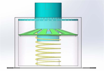
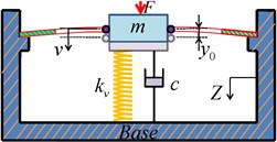
In this paper, a new QZS isolator including a vertical linear spring and a slotted conical disk spring is presented as shown in Fig. 1. The reason for taking a slotted conical disk spring as the negative structure is that it can supply a certain restoring force at the flatten state and produce axial nonlinear restoring force, which enables the isolator to support greater load and achieve the QZS property at the equilibrium position.
Most studies of QZS isolators assume that the system keep balance at the equilibrium where the dynamic stiffness equals zero. However, the overload or underload condition is more common in practical engineering, which motivates this paper to some extent. The aim of this paper is to investigate the characteristics of the QZS isolator and the influence of overload or underload on the isolation performance of the QZS isolator.
Fig. 1Prototype model of the proposed QZS isolator
2. Static characteristics of the QZS isolator
2.1. The slotted conical disk spring
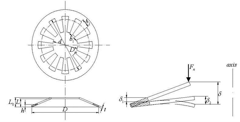
Consider a slotted conical disk spring loaded axially as shown in Fig. 2. It can be divided into a coned disk segment and a number of lever arm segments. The solution for the straight slotted disk spring is fully stated by Schremmer based on the theory of Almen and Laszlo [9]. Note that the total displacement includes the rigid displacement and bending displacement . The formulations between the axial applied force and the displacement are given by:
where is the Young’s modulus of the slotted conical disk spring, is the Poisson’s ratio and the other parameters are presented in Fig. 2. While the constants and are defined as:
The width ratio of slot tip to slot datum which is used to express the slot profile of a slotted conical disk spring does not significantly affect the nonlinear force-displacement [10]. Thus, simplified formula defining the slot profile with respect to the constant slot number , is introduced as follows:
Based on Eqs. (1) and (3), one can get the relationship between the total displacement and the rigid displacement :
When the coned disk segment of the slotted conical disk spring is in a horizontal line which means , the total displacement and the restoring force is (, ). It is worthy of note that the force-displacement curve is symmetric about the point as changes in the range [0, 2], i.e. changes in the range [0, 2]. It is convenient to define the following non-dimensional parameters:
Let , i.e. . By substituting the two equations and Eq. (5) given above into Eqs. (1a) and (4), the non-dimensional restoring force and the non-dimensional total displacement can be derived:
where is the non-dimensional force, is the non-dimensional displacement of the coned disk segment, and is the non-dimensional displacement of the slotted conical disk spring. In addition, can be derived as .
By differentiating Eq. (6a, b) with respect to the non-dimensional displacement separately, the non-dimensional stiffness of the slotted conical disk spring is obtained as:
Fig. 2The slotted conical disk spring under axial force
Considering the parameters , and , it can be found obviously that the stiffness is symmetric about and gets the minimum value at this position as changes in the range , i.e. changes in the range . Meanwhile, the slotted conical disk spring possesses continuous negative stiffness region when the parameters meet the condition .
2.2. Design and optimization of the QZS isolator
The schematic of the QZS isolator with a vertical linear spring and a viscous damper in parallel with a slotted conical disk spring acting as the negative stiffness structure is shown in Fig. 3. Here, the weight of the isolated mass is ignored and the stiffness of the linear spring is . As displayed in Fig. 3(a), the mass moves a certain total displacement from the initial position by the force . The restoring force can be expressed by:
By introducing the non-dimensional restoring force , and transforming the initial point to the symmetric point of the isolator following the procedure in Section 2.1. Then the non-dimensional restoring force can be obtained as:
where is defined as the stiffness ratio between the slotted conical disk spring and the linear spring, and the other parameters have the same meaning with that in Eq. (3). Differentiating Eqs. (9) and (6b) with respect to the non-dimensional displacement separately, one can get the non-dimensional stiffness of the isolator:
where is the non-dimensional stiffness.
Fig. 3Schematic representation of the QZS isolator. a) System balance at the position at which the dynamic stiffness is zero; b) overloaded system balance at a lower position; c) underloaded system balance at a higher position
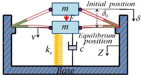
a)
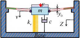
b)
c)
In operation, it is prospected that the isolator can reach the static equilibrium at the state the coned disk segment of the slotted conical disk spring is horizontal after loaded with a mass, in which , i.e. , and the stiffness of the isolator has a minimum value. Then setting the stiffness of the isolator to be zero at the equilibrium position provides that:
In addition to the isolator possessing the QZS property, it is desirable for it to own a wide range of non-dimensional total displacement from the equilibrium position for which the non-dimensional stiffness has a low value as well as changes slightly. By substituting and into Eqs. (6b) and (10) separately, these displacements are found to satisfy:
In this paper, the 50CrVA is used to be the material of the slotted conical disk spring, which has the following material properties: Young’s modulus , Poisson’s ratio and the ultimate stress . The configurative parameters , , and are chosen from the set , , and according to the practical engineering conditions [11]. Note that the stiffness ratio calculated using Eq. (11) should be positive and the non-dimensional stiffness should not be negative. The optimization criteria includes the condition that the largest displacement is achieved at which the stiffness of the isolator is equal to that of the linear spring, i.e. , and the requirement that the non-dimensional stiffness changes slightly with the tolerance of for in the region around the equilibrium position. In addition, the maximum stress of the slotted conical disk spring with the configurative parameters given above occurs at the lower outer edge and should not be larger than the ultimate stress [9].
The results of the optimization are , , and . The relationship between the non-dimensional stiffness and the non-dimensional displacement for the optimal parameters (Case 1) and other parameters satisfying the optimization criteria listed in Table 1 can be plotted in Fig. 4. The circles shown in Fig. 4 denote the maximum range given by Eq. (12) calculated at . It can be seen obviously that the optimized isolator possesses a very small stiffness in the region around the equilibrium position and a smaller stiffness for a larger displacement from the static equilibrium position.
Fig. 4Non-dimensional stiffness characteristics of the isolator for different parameters: ‘red line’ Case 1; ‘blue line’ Case2; ‘brown line’ Case 3; ‘green line’ Case 4
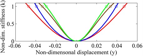
Table 1The configurative parameters of the QZS isolator
Case | ||||
1 | 0.83 | 0.1 | 0.01 | 0.022 |
2 | 0.83 | 0.1 | 0.02 | 0.031 |
3 | 0.7 | 0.18 | 0.01 | 0.031 |
4 | 0.61 | 0.25 | 0.01 | 0.036 |
3. Dynamic characteristics of the QZS isolator
3.1. Approximation of the restoring force
The restoring force of the isolator with respect to the total displacement could be derived by Eqs. (6) and (9), which is very complicated and can be expanded to the third order Taylor series at the zero stiffness position . The approximate restoring force is given by:
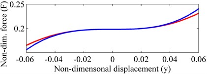
where and The exact restoring force expressed by Eqs. (6) and (9) and the approximate restoring force expressed by Eq. (13) are plotted in Fig. 5 both for the optimal parameters obtained in Section 2.2. Note that the error of the approximation depends on the non-dimensional displacement and less than 5 percent within the region .
Fig. 5Non-dimensional force-displacement of the QZS isolator: ‘red line’ exact expression; ‘blue line’ approximate expression
3.2. Dynamic modeling and solution
As shown in Fig. 3(a), the QZS isolator will keep balance at the equilibrium position when loaded with an appropriate mass, at which the dynamic stiffness is zero. Considering the practical applications, it is more possible that the isolator will balance at for overload or for underload as shown in Fig. 3(b) and 3(c) separately, owning an offset displacement . The static equilibrium equation of the QZS isolator can be derived as:
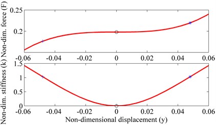
The non-dimensional force-displacement and stiffness characteristics of the isolator for overload and underload can be plotted in Fig. 6. It is evident that the equilibrium position for overload and underload will moves from the original position denoted by ‘o’ to a new position denoted by ‘*’ and ‘+’ separately, and the non-dimensional stiffness will not be zero at the new equilibrium position. The influence of overload and underload on the isolation performance of the isolator cannot be ignored. Go back to Fig. (3), the mass can represent a machine excited by the harmonic force or an equipment isolated from the base excitation . By applying the Newton’s second law of motion, one can get the dynamic equations of the system separately for the force and displacement excitations given above:
where is the relative displacement between the mass and the base, is the non-dimensional relative displacement. Introducing the non-dimensional parameters as follows:
and combing Eq. (14), Eqs. (15a) and (15b) can be rewritten separately as below:
Eq. (16) can be expressed by a uniform equation for simplicity:
where , , is the amplitude of the harmonic excitation, and for the force excitation; for the displacement excitation. By applying the transformation into Eq. (17) [12], one can get a Duffing equation under asymmetric excitation:
where the constant term . Using the Harmonic Balance Method (HBM), the approximate solution corresponding to the steady-state response in the region of the primary resonance is assumed to be:
Fig. 6Non-dimensional force-displacement and stiffness characteristics of the overloaded or underloaded system. ‘*’ Equilibrium position of the overloaded system shown in Fig. 3(b); ‘+’ equilibrium position of the underloaded system shown in Fig. 3(c)
Substituting Eq. (19) into Eq. (18), equating constant terms, and the coefficients of the terms containing and separately to zero, the steady-state response can be expressed by the constant term , the amplitude of the harmonic term and the phase as:
Combing Eqs. (20a), (20b) and (20c) gives the implicit equation for the amplitude of the constant term :
The implicit equations for the peak amplitude of the constant term for the force and displacement excitation, i.e. and , can be derived separately from Eq. (21):
Then the excitation frequency ratios that corresponding to the maximum responses can be expressed by:
The amplitude , the peak amplitude and of the harmonic term for the force and displacement excitation can be calculated separately from Eq. (20a). Eqs. (21), (22) and (23) are valid for the overloaded system balance at the position . The solution for the response of the underloaded system balance at another position can be obtained by transforming to in Eq. (21). According to the investigation of Kovacic et al. [13], it was found that the system excited by the asymmetric force may have a maximum number of one, three of five steady-state responses and multiple jumps for different combinations of excitation amplitudes.
For the system balance at the equilibrium position after loaded with an appropriate mass, the steady-state solutions of the system for both the force and displacement excitation can be derived by following the procedure above and setting . The dynamic equation is:
The implicit amplitude frequency equation is:
For the two types of excitation, the peak amplitude of the response and , and the excitation frequency ratios corresponding to the maximum responses can be obtained as follows:
The single degree of freedom (SDOF) system without the slotted conical disk spring can be regarded as the equivalent linear system (ELS). The dynamic equation for the ELS is:
The amplitude of the steady-state response for Eq. (28) can be derived as:
The optimal parameters , , , and the damping ratio are chosen to conduct the following investigation. Based on Descartes’ Rule of Signs [14] and the analysis above, the ways in which the maximum number of the steady-state values of and depend on the offset displacement and the excitation amplitude are shown in Fig. 7.
Fig. 7The maximum number of the steady-state amplitudes: one, three or five, as a function of the non-dimensional offset displacement y^0 and non-dimensional excitation amplitude β
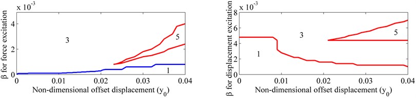
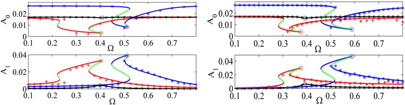
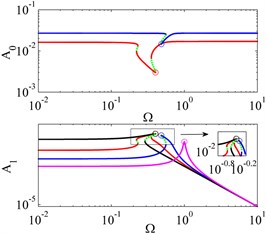
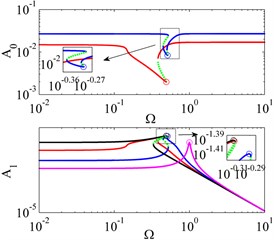
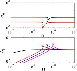
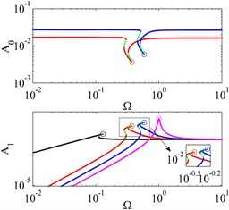
As shown in Fig. 7, there are a maximum number of one, three and five steady-state values for both force excitation and displacement excitation. For the force excitation, the FRCs with a maximum number of one, three and five steady-state values corresponding to , ; , ; , respectively, and for the displacement excitation, the FRCs with a maximum number of one, three and five steady-state values corresponding to , respectively are shown in Fig. 8 to illustrate these cases. In Fig. 8, the approximate solutions obtained by HBM are compared with the exact solutions obtained by numerical simulation. By using the MATLAB ode45 function and calculating the first harmonic from the Fourier series coefficients of the steady-state response, the exact solutions are obtained as shown in Fig. 8 with the symbol ‘*’. It can be obviously seen that both the constant term and the first harmonic term of the response are predicted reasonably well in the frequency range using the HBM.
Fig. 8FRCs of the constant term A0 and harmonic term A1 for the optimal parameters and ξ=0.03. a) For the force excitation: ‘black line’ y^0=1.7×10⁻², β=1×10⁻⁴; ‘red line’ y^0=1.7×10⁻², β=8×10⁻⁴; ‘blue line’ y^0=2.7×10⁻², β=1.2×10⁻³; b) For the displacement excitation: ‘black line’ y^0=1.7×10⁻², β=1×10⁻³; ‘red line’ y^0=1.7×10⁻², β=4.8×10⁻³; ‘blue line’ y^0=2.7×10⁻², β=4.8×10⁻³; ‘green dashed line’ unstable solution, ‘o’ peak amplitude and ‘*’ numerical solution
4. Effects of the offset displacement and excitation amplitude on the QZS isolator
To investigate the influence of the offset displacement and excitation amplitude on the FRCs and the transmissibility, the increasing values of the excitation amplitude are chosen to be , , , and when the value of the offset displacement is fixed to be or separately for the system excited by the harmonic force. And then the increasing values of the excitation amplitude are chosen to be , , , and when the value of the offset displacement is also fixed to be or separately for the system excited by the harmonic displacement. For the illumination convenience in the following sections, the system not being or being balance at the position at which the dynamic stiffness of the system is zero, i. e. the offset displacement or , are called system I and system II separately.
4.1. Effects on the FRCs for the force excitation and displacement excitation
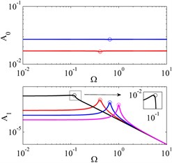
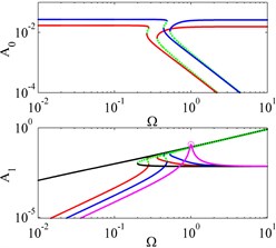
As shown in Fig. 9 and Fig. 10, the FRCs of system I and II are plotted separately for the both types of excitation, and that of the ELS is also plotted on the same figure for comparison. Note that the same values of the excitation amplitude and the damping ratio are chosen in the ELS.
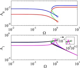
Fig. 9FRCs of system I, system II and their ELS for force excitations with different offset displacements and excitation amplitudes. ‘red line’system I with y^0=1.7×10⁻²,‘blue line’ system I with y^0=2.7×10⁻², ‘black line’ system II, ‘magenta line’ ELS, ‘green dotted line’ unstable solutions, ‘o’ peak amplitude of response
a)
b)
c)
d)
e)
By observing Fig. 9, for system I, a decrease in the offset displacement yields a decrease in both the amplitude of the constant term and the resonance frequency, and an increase in the peak amplitude of the harmonic term when the excitation amplitude is fixed. Note that the constant term disappears in system II. With the increase of the excitation amplitude, the FRCs of the ELS is shifted upwards in the whole frequency region and the peak amplitudes always occur at . For system I, the amplitude of the harmonic term is also increases. But the effect of the excitation amplitude on the constant term is only obvious around the resonance frequency, and larger excitation amplitude results in smaller peak amplitude of the constant term . For the frequency far away from the resonance frequency, the amplitude of the constant term does not change much and will approach to the value of the offset displacement . It is also worthy of note that the resonance frequency of system I decreases at first, increases later, and finally becomes larger than that of the ELS with the increasing excitation amplitude. For system II, larger excitation amplitude yields both larger amplitude of the response and the resonance frequency.
The excitation amplitude also effects the stiffness characteristics of system I and II obviously. Both system I and II approach to be a linear system if the excitation amplitude is small. When the excitation amplitude increases, system II always exhibits the hardening stiffness. However, with the increasing excitation amplitude, system I exhibits the softening stiffness, and then enters a region with the softening stiffness at first and the hardening stiffness later on. If the excitation amplitude keeps increasing, system I will only exhibit the hardening stiffness.
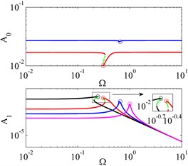
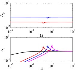
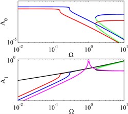
Fig. 10FRCs of system I, system II and their ELS for displacement excitations with different offset displacements and excitation amplitudes. ‘red line’ system I with y^0=1.7×10⁻², ‘blue line’ system I with y^0=2.7×10⁻², ‘black line’ system II, ‘magenta line’ ELS, ‘green dotted line’ unstable solutions, ‘o’ peak amplitude of response
a)
b)
c)
d)
e)
In addition, another conclusion about the three systems can be drawn. For the same excitation amplitude, the amplitude of the harmonic term in system II is larger than that in system I and the amplitude of the harmonic term in system I is larger than that in ELS at lower frequencies; but when the excitation frequency is around the resonance frequency of the ELS, the amplitude of the harmonic term in system II becomes smaller than that in system I and the amplitude of the harmonic term in system I becomes smaller than that in ELS; and at higher frequencies the amplitudes of the harmonic term in the three systems are almost the same.
Fig. 10 is for the displacement excitation, of which the vertical coordinate represents the relative displacement. Unlike the FRCs for the force excitation, the amplitudes of the harmonic term in system I, II and the ELS will approach to the excitation amplitude with the increasing excitation frequency. The amplitude of the harmonic term in system II reaches the excitation amplitude at the lower frequency than that in system I, and the amplitude of the harmonic term in system I reaches the excitation amplitude at the lower frequency than that in ELS. When the excitation amplitude is relatively large, unbounded responses will occur for both system I and II which is not observed in Fig. 9.
4.2. Definition of the transmissibilities
Force transmissibility for the force excitation and absolute displacement transmissibility for the displacement excitation are the key indexes to evaluate the vibration isolation performance of a vibration isolator [15]. According to the study of Ravindra and Mallik [12], it is concluded that the nonlinear system with asymmetric restoring force may not perform satisfactorily for the displacement excitation by using the absolute displacement transmissibility to evaluate the isolation performance. Therefore, the absolute acceleration transmissibility for the displacement excitation is also introduced to evaluate the isolation performance for the displacement excitation.
4.2.1. Force transmissibility
The force transmissibility is defined as the ratio of the amplitude of the non-dimensional dynamic force transmitted to the base, to the amplitude of the non-dimensional excitation force. It is given by:
where , is the non-dimensional elastic force and is the non-dimensional damping force.
For system I, the solution of Eq. (17) can be expressed by [16]:
where the constant term .
The non-dimensional elastic force is:
By substituting Eq. (31) into Eq. (32), one can get the implicit expression of the non-dimensional elastic force:
where:
Only considering the dynamic force here, then the force transmissibility of system I can be expressed by:
For system II, the force transmissibility is determined by [2]:
Using Eq. (29), the force transmissibility of ELS can be derived as:
4.2.2. Absolute displacement and acceleration transmissibility
The absolute displacement transmissibility is defined as the ratio between the amplitude of the non-dimensional absolute displacement and amplitude of the non-dimensional excitation displacement. It is given by:
For system I, one can get the expression of the absolute displacement of the mass by employing Eq. (18):
The absolute displacement transmissibility can be defined as:
Then the absolute acceleration transmissibility of system II can be derived as:
where in Eqs. (39) and (40) can be obtained by Eq. (20b).
For system II, the absolute displacement and acceleration transmissibility have the same expression as:
noting that the in Eq. (41) should be obtained by setting in Eq. (20b).
For the ELS, the absolute displacement and acceleration transmissibility are also the same with the force transmissibility and given by:
4.3. Effects on the tranmissibilities
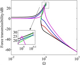
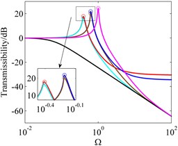
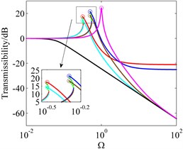
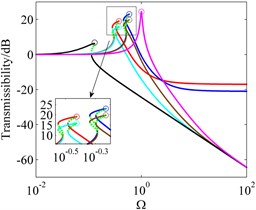
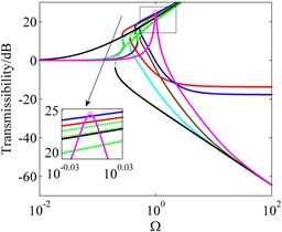
The force transmissibility is plotted in Fig. 11. The absolute displacement and acceleration transmissibility are plotted in Fig. 12. All the transmissibility results are plotted in dB, i.e. as , and . As shown in Fig. 11 and Fig. 12, both system I and II will exhibit superior or inferior isolation performance to the ELS depending on the excitation frequency range and the excitation amplitude.
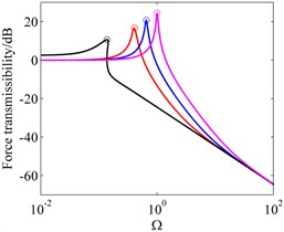
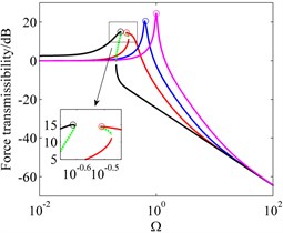
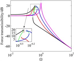
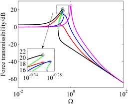
Fig. 11Force transmissibility of system I, system II and their ELS for displacement excitations with different offset displacements and excitation amplitudes. ‘red line’ system I with y^0=1.7×10⁻², ‘blue line’ system I with y^0=2.7×10⁻², ‘black line’ system II, ‘magenta line’ ELS, ‘green dotted line’ unstable solutions, ‘o’ peak amplitude of transmissibility
a)
b)
c)
d)
e)
By observing Fig. 11, for system I, a decrease in the offset displacement yields a decrease in both the peak amplitude of the force transmissibility and the resonance frequency, and the transmissibility curve approaches to the transmissibility curve of system II. If the force excitation amplitude is relatively large, the peak amplitude of the force transmissibility and the resonance frequency in system II are larger than that in system I. However, system II will present better isolation performance compared with system I when the excitation frequency exceeds the resonance frequency. For system II, larger excitation amplitude results in both larger peak amplitude of the force transmissibility and the resonance frequency. By combing the characteristics of the stiffness and resonance frequency for different excitation amplitudes in Section 4.2, it is found that the peak amplitude of the force transmissibility of system I decreases at first, increases later, and finally becomes larger than that of the ELS with the increasing excitation amplitude. For the same excitation amplitude, the force transmissibility of system II is larger than that of system I and the force transmissibility of system I is larger than that of the ELS at lower frequencies; but when the excitation frequency is around the resonance frequency of the ELS, the force transmissibility of system II becomes smaller than that of system I and the force transmissibility of system I becomes smaller than that of ELS; and at higher frequencies the force transmissibility of the three systems are almost the same.
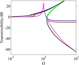
Different from the force transmissibility for the force excitation, both system I and II have unbounded absolute displacement and acceleration transmissibility as shown in Fig. 12. For system I, the absolute acceleration transmissibility is always better than the absolute displacement transmissibility. For the same excitation amplitude, the interactive characteristics of both the absolute displacement and acceleration transmissibility among system I, II and their ELS are same with that of the force transmissibility when the excitation frequency is lower or around the resonance frequency of the ELS. However, at higher frequencies the absolute acceleration transmissibility of the three systems are almost the same while the absolute displacement transmissibility of system I is larger than that of system II and the ELS. And the absolute displacement transmissibility of system I increases with the increasing excitation amplitude at higher excitation frequencies.
Fig. 12Absolute displacement and acceleration transmissibility of system I, system II and their ELS for offset displacements with different equilibrium positions and excitation amplitudes. ‘red line’ absolute displacement transmissibility of system I with y^0=1.7×10⁻², ‘cyan line’ absolute acceleration transmissibility of system I with y^0=1.7×10⁻², ‘blue line’ absolute displacement transmissibility of system II with y^0=2.7×10⁻², ‘brown line’ absolute acceleration transmissibility of system II with y^0=2.7×10⁻², ‘black line’ system II, ‘magenta line’ ELS, ‘green dotted line’ unstable solutions, ‘o’ peak amplitude of transmissibility
a)
b)
c)
d)
e)
5. Conclusions
In this paper, a QZS isolator fabricated by adding a slotted conical disk spring in parallel with a vertical linear spring is presented. Firstly, the geometrical configuration for designing the unique feature of quasi-zero stiffness is described and the corresponding mathematical modeling is formulated. The configurative parameters are optimized to achieve a wide range of the displacement from the equilibrium position for which the stiffness has a low value and changes slightly.
Secondly, the system of an offset equilibrium position for overloaded or underloaded, and the system of an equilibrium position in which the dynamic stiffness is zero for loaded with an appropriate mass are studied. The primary resonance response for the force excitation and displacement excitation is separately derived by employing the HBM and confirmed by the results of numerical simulation. The ways in which the maximum number of the steady-state values depends on the offset displacement and the amplitude of the two types of excitation are also separately reported.
Thirdly, the frequency response curves of the two kinds of system for the two types of excitation have been plotted. The frequency response curves of their equivalent linear system are plotted in the same figure for comparison. The overloaded system can exhibits purely softening, mixed softening-hardening and purely hardening with the increasing excitation amplitude. It can be summarized that both larger offset displacement and excitation amplitude result in a higher resonance frequency.
Finally, the force transmissibility, the absolute displacement and acceleration transmissibility are chosen to evaluate the isolation for the two kinds of systems and compared with their equivalent linear system. It can be concluded that adding the slotted conical disk spring acting as the negative structure to a linear spring is a feasible way to achieve the wider isolation frequency region and smaller transmissibility. Additionally, an effective way to achieve better isolation performance is applying the QZS isolator in the conditions that the mass differs less with its load capability and the excitation amplitude is not too large.
References
-
Rivin E. I. Passive Vibration Isolation. ASME Press, New York, 2001.
-
Carrella A. Passive vibration isolators with high-static-low-dynamic-stiffness. Ph. D. Thesis, ISVR, University of Southampton, 2008.
-
Ibrahim R. A. Recent advances in nonlinear passive vibration isolators. Journal of Sound and Vibration, Vol. 314, 2008, p. 371-452.
-
Alabuzhev P., Gritchin A., Kim L., Migirenko G., Chon V., Stepanov P. Vibration Protecting and Measuring Systems with Quasi-Zero Stiffness. Hemisphere, New York, 1989.
-
Platus D. L. Negative-stiffness-mechanism vibration isolation systems. Proceedings of SPIE, Vol. 3786, 1999, p. 98-105.
-
Zhang J., Li D., Dong S. An ultra-low frequency parallel connection nonlinear isolator for precision instruments. Key Engineering Materials, Vol. 257-258, 2004, p. 231-236, (in Chinese).
-
Le T. D., Ahn K. K. A vibration isolation system in low frequency excitation region using negative stiffness structure for vehicle seat. Journal of Sound and Vibration, Vol. 330, 2011, p. 631-6335.
-
Liu X., Huang X., Hua H. On the characteristics of a quasi-zero stiffness isolator using Euler buckled beam as negative stiffness corrector. Journal of Sound andVibration, Vol. 332, 2013, p. 3359-3376, (in Chinese).
-
Schremmer G. The slotted coned disk spring. Journal of Engineering for Industry, Trans. of the ASME, 1973, p. 765-770.
-
Frawazi N., Lee J. Y., Oh J. E. A load-displacement prediction for a bended slotted disc using the energy method. Proceedings of the Institution of Mechanical Engineers, Part C: Journal of Mechanical Engineering Science, Vol. 2126, 2012, p. 2126-2137.
-
Zhang Y., Liu H., Wang D. Spring Manual. China Machine Press, Beijing, 2008, (in Chinese).
-
Ravindra B., Mallik A. K. Performance of non-linear vibration isolators under harmonic excitation. Journal of Sound and Vibration, Vol. 170, Issue 3, 1994, p. 325-337.
-
Kovacic I., Brennan M. J., Lineton B. On the resonance response of an asymmetric Duffing oscillator. International Journal of Non-Linear Mechanics, Vol. 43, 2008, p. 858-867.
-
Korn G. A., Korn T. M. Mathematical Handbook for Scientists and Engineers. McGraw-Hill, New York, 1961.
-
Guo P., Lang Z., Peng Z. Analysis and design of the force and displacement transmissibility of nonlinear viscous damper based vibration isolation systems. Nonlinear Dynamics, Vol. 67, 2012, p. 2671-2687.
-
Liu X., Huang X., Zhang Z., Hua H. Influence of excitation amplitude and load on the characteristics of quasi-zero stiffness isolator. Journal of Mechanical Engineering, Vol. 49, Issue 6, 2013, p. 89-94, (in Chinese).
About this article

This research was supported in part by the National Science and Technology Major Project of China (Grant No. 2012ZX10004801-002-013).
