Near-field beamforming performance analysis for acoustic emission source localization

1. Introduction

Acoustic Emission (AE) is a phenomenon of stress wave radiation caused by a dynamic reconstruction of material’s structure that accompanies processes of deformation and fracture [1]. Material deformation and crack propagation under stress is an important mechanism of structural failure. And like this damage source directly related to deformation and fracture mechanisms is known as AE source [2]. The AE technique, in the early 1950s, started with Kaiser’s research done in Germany. And in the following decades, AE technique had been improved continuously. Now, AE technique is used as a non-destructive testing tool to evaluate structural damage and has its potential advantages in dynamic damage monitoring and source localization, such as fatigue crack growth [3, 4]. Due to its potential advantages, AE technique has led to many applications in a variety of fields such as petrochemical industry, aerospace industry and detection of metal processing, etc. [5, 6].

AE source localization is an important step in whole damage identification process, by which the accurate AE source location can indicate information about the characteristic of the damage and even the size of the crack with relatively few sensors on large and complex structures. Current localization of AE sources is normally performed by using the time difference of arrival (TDOA) technique which uses the propagation velocity in a material to derive the source location in one, two or three dimensions from the arrival delay between sensors based on first threshold crossing. However, when the AE wave propagates in the solid medium, the AE signals may be significantly affected by multi-mode, dispersion, energy attenuation and other factors, which make it difficult to determine the arrival time accurately. Besides, when there is more than one AE source, the arrival time information may be confused, which is also one key problem of TDOA [7, 8]. To make the localization simple but effective, AE beamforming was introduced to localize AE source by McLaskey et al. [9] in civil engineering field applications on large plate-like reinforced concrete structures. Considering the specimens estimated in their work are large reinforced concrete structures in civil engineering while the structures generally seen in aviation fields are thin plates and shells, He et al. [10, 11] explored the possibility of AE source localization in a thin plate by near-field AE beamforming techniques and improved localization accuracy with two uniform linear arrays. Nakatani and Kundu et al. [12-14] studied AE source localization on an anisotropic structure with a beamforming array technique, which expanded AE beamforming applications in composite materials.

Although AE beamforming has been successfully used in damage localization by several scholars, its performance has not been studied in depth. Beamforming performance is mainly effect by some parameters such as sensor arrays, localization velocity, the maximum diameter of the array and the sensor spacing etc. Research on acoustic beamforming localization performance has been done deeply by many scholarships [15, 16]. However, the propagation characteristic of AE signal in solid is very different from acoustic signal in air, such as high frequency, multi-mode and dispersion, so some previous experiences on the acoustic beamforming may not be suitable for AE beamforming. For example, dispersion means that velocity of AE signal is not easy to calculate correctly, this can cause localization errors. Therefore, knowing how to use AE beamforming and its performance are crucial.

This article aims to study how beamforming with different parameters, including sensor arrays, localization velocity, the maximum diameter of the array and the sensor spacing, affect localization performance. AE beamforming with different array parameters consisting of different sensor arrays and sensor spacing is implemented. In addition, in order to study AE beamforming localization performance more aviable, an improved FE simulation method is proposed to get pure AE signal under different array parameters and analyze the propagation characteristics of AE signal. On basis of this, effect of different parameters on the AE beamforming localization performance is analyzed.

2. AE beamforming method

Beamforming is a signal processing technique used in sensor arrays for directional signal transmission or reception [17]. It is also used in acoustic source localization and develops several localization algorithms. For AE source localization, delay-and-sum algorithm is usually used. Delay-and-sum is a simple and effective array signal processing algorithm utilized in beamforming techniques [18]. Considering the distance between AE source and array of sensors, the analysis schemes based on beamforming techniques can be divided into near-field and far-field methods. A common rule of thumb is that the near-field sources are located at a distance of:

where $r$ is the radial distance from an arbitrary array origin, $L$ is the largest array dimension and $\lambda$ is the operating wavelength [19]. The acquired wavefront from the sound source, in such conditions, is assumed spherical due to the transmission characteristics of waves. The far-field sources refer to those at locations $r$ larger than$r>2L^2/\lambda$, of which the wavefront is usually assumed planar.

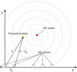
The goal of present study is to estimate the source localization performance of thin plates or shells in aviation fields. The beamforming analysis for such structures is usually categorized into near-field, based on the aforementioned rule. The basic principle of near-field beamforming based on the delay-and-sum algorithm is illustrated in Fig. 1. The incident waves are spherical and thus the array output of these waves can be expressed by:

where $\overrightarrow{r}$ represents the distance of the focus to the reference point. The reference point may be arbitrary and it is the first sensor point on the left side in the Fig. 1. $M$ is the number of the sensors and $w_m$ is the weighting coefficient applied to the channel of sensor $m$. The variable $x_m\left(t\right)$ represents the signal acquired from the No. $m$ sensor and ${\mathrm{\Delta }}_m\left(\overrightarrow{r}\right)$ indicates the individual time delay of No. $m$ sensor to the reference point. Though different $w_m$ are adopted in the formula to control the beamwidth and sidelobes of the sensor array, a constant $w_m\equiv \text{1}$ is used in this work. And the time delay ${\mathrm{\Delta }}_m\left(\overrightarrow{r}\right)$ is adjusted in delay-and-sum beamforming in such a way that signals associated with a spherical wave, incident from the real source, are aligned in time before they are summed when the focus is located at the real source [20]. Conversely, signals are not able to be aligned before summation if positions of the focus and real source are not coincident. As shown in Fig. 1, the time delay ${\mathrm{\Delta }}_m\left(\overrightarrow{r}\right)$ is obtained by:

where ${\mathrm{\Delta }}_m\left(\overrightarrow{r}\right)$ represent the distances of reference point to No. $m$ sensor. And $c$ is the propagation velocity of signal.

Fig. 1Illustration of delay-and-sum beamforming

The general assumption of beamforming is that the received wave is a plane wave or a spherical wave. Most researches of beamforming are for acoustic field, but rarely for AE wave field. So the further research on AE beamforming localization performance is needed. Some characteristic parameters that represent the localization performance of delay-and-sum consist of localization accuracy, resolution, and the main lobe width etc. [21]. When the focusing direction of array is consistent with the sound source direction, the energy output of the array is enhanced and the maximum value is obtained, referred to as main lobe, otherwise, energy attenuation, called side lobe. A good array should have a smaller width of the main lobe and smaller side lobe level, which will have a higher resolution and excellent anti-interference ability. The width of the main lobe is given by:

where $\alpha =$ 1 is for the linear array, $\alpha \approx$ 1.22 is for the circular array, and $D$ is the maximum diameter of array [20].

The resolution is mainly reflected in the width of the main lobe, the narrower the main lobe is, the better the resolution is, and it usually describes the ability to distinguish waves incident from directions close to each other. According to Rayleigh criterion, the resolution of beamforming is given by:

where $z$ is the distance between the sound source and the array. $\theta$ is the off-axis angle. Obviously, resolution is related to the maximum diameter of array $D$, the off-axis angle $\theta$, and signal frequency. The larger $D$ is, and the smaller $\theta$ is, the better resolution is.

These parameters are usually affected by the array of beamforming which is composed by a number of sensors arrayed according to the spatial geometric position. It is obviously that the array parameters include spacing between sensors, the pore size of the array, the spatial distribution patterns of the sensors, the number of the sensors and other geometrical parameters.

To obtain AE signals under the condition of different array parameters, this paper uses an improved finite element (FE) simulation method, by which the propagation characteristics of AE signals is investigated and the performance of AE beamforming can be analyzed comprehensively.

3. AE signal simulation based on FEM

The FE simulation model is a homogeneous plate with properties of steel and specifically elasticity modulus, and parameters are set as follows: $E=\text{209×}{\text{10}}^{\text{9}}\text{N/}{\text{m}}^{\text{2}}$, Poisson’s ratio $\upsilon =\text{0.3}$; density $\rho =\text{7800}\text{Kg/}{\text{m}}^{\text{3}}$. Simulation process is achieved with ABQUS.

In the frequency range of interest, only the zero-order symmetric mode, $S_0$, and anti-symmetric mode, $A_0$, are present. These two modes are selectively excited in the model by applying appropriate nodal loads. For a maximum frequency of 200 kHz, the minimum wavelength is for $A_0$ and it is given by, ${\lambda }_{min}=c_s/f_{max}=\text{15.7}\text{mm}$, considering a theoretical phase velocity of shear wave $c_s=$3230 m/s. In present study the value of ${\lambda }_{min}$ is assigned as 20 mm.

The package used in the present study, ABAQUS/EXPLICIT, uses an explicit integration based on a central difference method [22]. The stability of the numerical solution is dependent upon the temporal and the spatial resolution of the analysis.

To avoid numerical instability, ABAQUS/EXPLICIT recommends a stability limit for the integration time step ${\mathrm{\Delta }}_t$ equal to:

The maximum frequency of the dynamic problem, $f_{max}$, limits both the integration time step and the element size. A good rule is to use a minimum of 20 points per cycle at the highest frequency, that is:

The size of the finite element, $l_e$, is typically derived from the smallest wavelength to be analyzed, ${\lambda }_{min}$. For a good spatial resolution 20 nodes per wavelength are normally required:

From Eq. (8), the corresponding limit on the element size is $l_e=$1 mm. According to Eq. (7), this transient problem is solved with an integration time step, ${\mathrm{\Delta }}_t=$0.25 μs.

In the laboratory, the AE waves in plates are generated passively by using a mechanical pencil lead break input, and actively using a surface bonded piezoelectric actuator [23]. To model impact, delamination, or crack propagation, a transient excitation such as a delta or step function is needed. In order to stimulate AE signal, the past used a couple forces with triangular (or rectangular) forcing function $f\left(t\right)$ acting at two nodes of the finite element model as buried dipole source, then by adjusting the size of the force and time, AE signals with different main frequency component can be obtained. Usually the total distance of the two points acting as buried dipole source is 1 mm with 1 N force magnitude [24, 25]. In this paper, on the basis of previous methods, another couple of forces are also added perpendicular to the original. It is shown in Fig. 2. The chosen excitation time investigated is 2.5 μs. The sampling rate of 5 MHz is sufficient to resolve the observed signals frequency content in the range up to a maximal frequency of 0.2 MHz. Simulation results are shown in Fig. 3. After the improvements, the AE signal is closer to real propagation characteristics.

Fig. 2The acting forces and time function of applied load

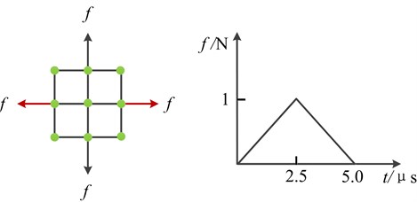
Fig. 3FE simulation results of AE signal: a) Wave propagation scenes at 60 μs with only one couple of axisymmetric forces; b) Wave propagation scenes at 60 μs with two couples of axisymmetric forces

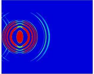
a)

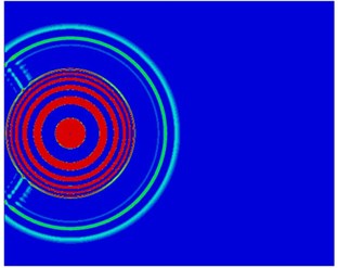
b)

4. The localization performance of beamforming with different parameters

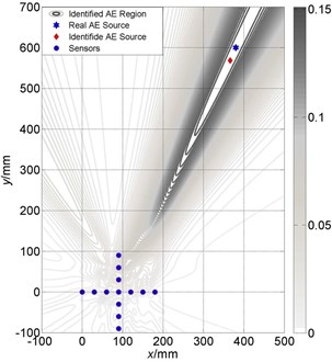
The FE simulation model is a steel plate has the dimensions of 1000 mm length, 800 mm width and 5 mm height. Fig. 4 shows the different sensor arrays with spacing of 30 mm (circular array is approximately equal to 30 mm). Linear array and cross array consist of the sensors on straight line. Circular arrays are made of the sensors on circle line. Different array parameters can be obtained by choosing different number of sensors. Coordinate system is established with $x$ and $y$, and origin of coordinate is on the center of the leftmost sensor. The AE sources are respectively marked with 1# (30 mm, 300 mm), 2# (90 mm, 600 mm) and 3# (380 mm, 600 mm).

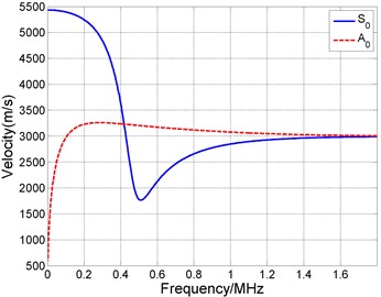
The propagation velocity of the AE signals is 5390 m/s by TDOA. The waveforms and frequency spectrum of one signal acquired by FE simulation are shown in Fig. 5. It can be seen that most energy of signals are within the range of frequencies less than 0.4 MHz. Consequently, it has been known that most waves transmitted in a thin steel plate are $A_0$ and $S_0$ waves. Fig. 6 shows the relation between frequency and propagation velocities of $S_0$ and $A_0$ waves.

This paper employs delay-and-sum beamforming to localize AE sources only with $S_0$ wave which can be obtained by setting a small threshold. And beamforming localization performance is discussed from the following four aspects.

Fig. 4Sensor arrays and AE source locations

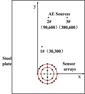
Fig. 5The waveforms and frequency spectrum of AE signal received by one sensor

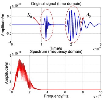
Fig. 6Dispersion curves of S0 and A0 waves in 5 mm steel plate

4.1. Beamforming arrays

Beamforming has the following basic arrays, linear array, circular array, and cross array [26]. The parameters of different arrays are shown in Table 1. With delay-and-sum beamforming for AE source identification, the localization results of three AE sources identified by different arrays are shown in Table 2.

Table 1The parameters of different arrays

Sensor arrays	Number of sensors	Maximum diameter (mm)
Linear array (large)	7	180
Linear array (small)	5	120
Cross array (large)	13	180
Cross array (small)	9	120
Circular array (large)	12	180
Circular array (small)	8	120

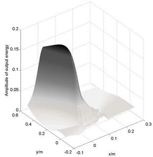
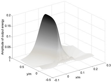
The localization results of AE source 1# with linear array are given in Fig. 7. The contours in figures represent the outputs of array based on beamforming and the maximal output region is the identified AE region, in which the focused position with maximum energy value is the identified AE source. The zone of the maximum peak is the main lobe width of the main lobe, and the other small peak regions are side lobes which have bad influence on localization accuracy. The smaller the width of the main lobe is, the higher localization accuracy is. And the more clearly distinction between main lobe and side lobe is, the better localization performance is. The star “*” is the real location of AE source, and the diamond “◇” is the identified AE source.

Table 2The localization results of different arrays

Sensor arrays	AE sources	Localization results ($x$, $y$) (mm)
Linear array (large)	1#	(30, 301)
	2#	(90, 604)
	3#	(384, 617)
Cross array (large)	1#	(30, 300)
	2#	(90, 601)
	3#	(383, 602)
Circular array (large)	1#	(30, 301)
	2#	(90, 602)
	3#	(385, 607)

Fig. 7Energy output contours of linear array (big) localization result at AE source 1#: a) three-dimensional contour output picture; b) planar output picture

a)

b)

It is clearly seen from Table 2 that, with the same array diameter and sensor spacing, all three arrays can localize the real AE sources approximately. These arrays all have wonderful localization accuracy at AE source 1# which is close to the center of the array and AE source 2# which is on the center line of the array. The localization accuracy of cross array and circular array are superior to the linear array at AE source 3# that is away from the sensor arrays and has a large deviation from the center line of the array. However, the linear array with a minimum number of sensors and good performances has more advantages than the circular array and cross array in practical engineering applications.

4.2. The impact of selected velocity on the localization accuracy

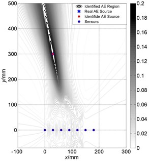
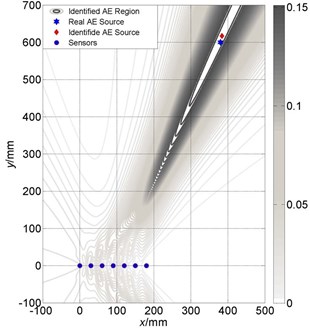
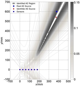
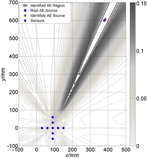
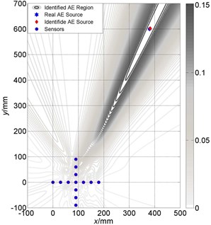
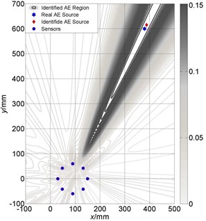
For the acoustic signal in the air, the propagation velocity is almost fixed. However, the AE signal have dispersion, that is, components of different frequency have different propagation velocities. In this paper, the AE signal is obtained by finite element simulation, in which the velocity of main frequency components can be calculated exactly, but in practical engineering applications, the velocity is not accurate. From Eq. (6), it is shown that ${\mathrm{\Delta }}_m\left(\overrightarrow{r}\right)$ is affected by velocity, $c$. Therefore, velocity is influential on the localization results and knowing its impact on localization accuracy is necessary. Figs. 8-10 show the impact of velocities on the localization accuracy of three different arrays at AE source 3#. It can be seen that, for linear array, the localization accuracy of x-direction is affected a little, while $y$-direction has large deviation. And, for the cross array, the localization accuracy on both of $x$ and $y$ directions are stable. However, the localization accuracy of the circular array is affected largely by velocity.

Fig. 8Localization results comparison between different velocities of linear array: a) localization with accurate velocity; b) deviation from accurate velocity with 300 m/s

a)

6

Fig. 9Localization results comparison between different velocities of cross array: a) localization with accurate velocity; b) deviation from accurate velocity with 300 m/s

a)

b)

Fig. 10Localization results comparison between different velocities of circular array: a) localization with accurate velocity; b) deviation from accurate velocity with 300 m/s

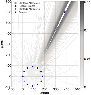
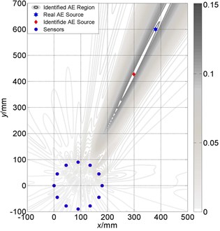
Fig. 11Localization results comparison between large and small size of linear array: a) Localization results of linear array (small) is (386 mm, 624 mm); b) Localization results of linear array (large) is (384 mm, 617 mm)

a)

b)

Fig. 12Localization results comparison between large and small size of cross array: a) Localization results of cross array (small) is (386 mm, 609 mm); b) Localization results of cross array (large) is (383 mm, 603 mm)

a)

b)

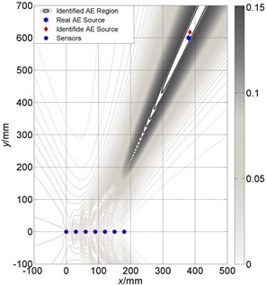
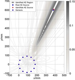
Fig. 13Localization results comparison between large and small size of cross array: a) Localization results of round array (small) is (388 mm, 616 mm); b) Localization results of round array (large) is (385 mm, 608 mm)

a)

b)

4.4. The sensor spacing

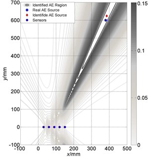
Sensor array requires spatial sampling of the input signal as the same as time domain sampling theorem which should ensure that frequency aliasing does not occur to generate pseudo signals. For beamforming method, this requirement becomes that the pseudo main lobe should not appear during localization process. Appearance of pseudo main lobe is directly related to the distance between sensors. If the sensor spacing is too large, it may produce the big side lobes (the false main lobes), even a pseudo AE source. From Fig. 14, it can be seen that side lobes become bigger when the sensor spacing is changed from 30 mm to 60 mm.

Fig. 14Localization results comparison between different sensor spacing of linear array: a) the distance between sensors is 30 mm; b) the distance between sensors is 60 mm

a)

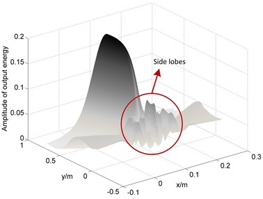
b)

5. Conclusions

The AE propagation characteristics are analyzed on the views of establishing the finite element model of AE signal propagation in the plate. The influences of some parameters on AE beamforming localization performance are investigated through simulation of AE signals, such as the AE sensor arrays, the selected velocity, the maximum diameter of array, and the sensor spacing.

According to the results, the following conclusions can be obtained:

1) All three kinds of arrays can get a good accuracy at the AE source which is close to the center of the array or is on the center line of the array. The localization accuracy of cross array and circular array are superior to the linear array at AE source which is away from the sensor arrays and has a large deviation from the center line of the array.

2) When AE beamforming is used, especially AE source is farther away from the array center, localization velocity has an influence on the localization accuracy. From different types of three arrays, cross array has the better stability and circular array is affected largely by localization velocity.

3) For these three arrays, with the same sensor spacing, the larger maximum dimension of the array, the better localization accuracy.

4) When the sensor spacing becomes large, the side lobes of array will become big.

5) According to conclusion (1-4), the appropriate array parameters in engineering practice are recommended: a) Arrangement of linear array is simple, and the number of linear array is the least. In most cases, linear array can meet AE localization in practical engineering applications. So it should be the priority for selection; b) When high-precision localization is required, the cross array and circular array should be considered. The circular array has a better main lobe and smaller side lobe, but its localization accuracy easily effected by selected velocity. If the AE wave velocity can be calculated exactly, the circular array is a good choice. The cross array has the best localization accuracy and can reduce the effect of localization velocity. If components of AE signal and the velocity can’t be calculated exactly, the cross array should be considered; c) The sensor spacing should be selected as small as possible to ensure no pseudo localization sources.